Welcome

Welcome to my website, hope you enjoy it, most of the notes are listed below:

Some backgrounds:

1. Probability (1)
2. Probability (2)
3. Probability (3)
4. Advanced Probability (1)
5. Advanced Probability (2)
6. Calculus (1)
7. Calculus (2)
8. Backpropagation in CNN
9. RNN
10. Real Analysis (1)
11. Real Analysis (2)
12. Real Analysis (3)
13. Real Analysis (4)
14. Measure Integral and Real Analysis (1)
15. Measure Integral and Real Analysis (2)
16. Measure Integral and Real Analysis (3)
17. Measure Integral and Real Analysis (4)
18. Time Series (1)
19. Time Series (2)
20. Time Series (3)
21. Linear Algebra (1)
22. Linear Algebra (2)
23. Linear Algebra (3)
24. Linear Algebra (4)
25. Linear Algebra (5)
26. Fourier Analysis

Some RL backgrounds:

1. MDP
2. Bellman Equations
3. Bellman Optimality Equations
4. Dynamic Programming
5. Value Iteration
6. Policy Iteration
7. Learning From Stream of Data
8. Monte Carlo Methods
9. Temporal Difference Learning
10. SARSA
11. Q Learning
12. Value Function Approximation (1)
13. Value Function Approximation (2)
14. Policy Gradient (1)
15. Policy Gradient (2)
16. Policy Gradient (3)
17. Average Reward Setting (Under Construction)
18. Semi MDP (Under Construction)

Some interesting RL algorithms:

1. DPG
2. DDPG
3. DDQN
4. TD3
5. Dueling DQN
6. TRPO
7. PPO
8. Prioritized Experience Replay
9. Intrinsic Motivation
10. Go Explore
11. Natural Actor Critic (Under Construction)
12. Off Policy Actor Critic (Under Construction)
13. SAC (Under Construction)

Some Deep Learning algorithms and models:

1. Dropout
2. Batch Normalization
3. Layer Normalization
4. Xavier Initialization
5. Kaiming Initialization
6. LReLU
7. Alex Net
8. Overfeat (Under Construction)
9. VGG (Under Construction)
10. Momentum
11. Basic Adaptive LR Methods
12. Adam
13. Attention
14. TCN
15. Transformer

Some old school ML algorithms:

1. PCA
2. Logistic Regression
3. Naive Bayes
4. Decision Trees
5. Random Forest (Under Construction)
6. AdaBoost
7. GBDT
8. K-means
9. KNN (Under Construction)
10. SVM (Under Construction)
11. EM Algorithm
12. ROC
13. LGBM
14. Graphical Models (Under Construction)
15. Sequential Data Modeling (Under Construction)

Some CS:

1. LeetCode (1)
2. LeetCode (2)
3. LeetCode (3)
4. LeetCode (4)
5. Heaps
6. Sorts
7. Trees

Change of Variable

The change of variable formula is:

\[\int^{a}_{b} f(x) dx = \int^{y(b)}_{y(a)} f(g(y)) \frac{dg}{dy} dy\]

where \(x = g(y)\).

Suppose \(X\) is a probability distribution with density \(p_X(x)\) and \(Y = g(X) \implies X = g^{-1}(Y)\). For the probability of \(Y\) we have \(P(g(a) \leq Y \leq g(b)) = P(a \leq X \leq b)\). Then,

\[P(g(a) \leq Y \leq g(b)) = P(a \leq X \leq b) = \int^{a}_{b} p_X(x) dx = \int^{g(b)}_{g(a)} p_X(g^{-1}(Y))|\frac{dg}{dy}| dy\]

That is:

\[p_Y(y) = p_X(g^{-1}(Y))|\frac{dg}{dy}|\]

Reference

https://www.cl.cam.ac.uk/teaching/0708/Probabilty/prob11.pdf

Fisher Information

Definition

The score function is defined as:

\[s(\theta; X) = \frac{\partial \log f(X; \theta)}{\partial \theta}\]

When it equals to \(0\), we have the maximum likelihood estimator:

\[s(\hat{\theta}; X) = 0 \implies \hat{\theta} = \arg\max_{\theta} \log f(X; \theta)\]

The expectation of the score function evaluated at the true parameter value \(\theta_0\) is:

\[E_{\theta_0}[s(\theta; X) |_{\theta = \theta_0}] = \int_{X} f(X| \theta_0)\frac{\partial f(X; \theta_0) / \partial \theta_0}{f(X| \theta_0)} dx = 0\]

This makes sense, since the true parameter should have gradient zero for all values of \(X\). Now we are interested in the curvature information around the score function of true parameter:

\[-E_{\theta_0} [\frac{\partial{s(\theta; X)}}{\partial \theta} |_{\theta = \theta_0}] = E_{\theta_0}[s(\theta ; X)^2 |_{\theta=\theta_0}] = \text{Var}_{\theta_0}(s(\theta ; X) |_{\theta=\theta_0})\]

Thus, the curvature information coincides with the variance of score function at the true parameter value. This is called the fisher information at parameter \(\theta_0\):

\[I(\theta_0) = \text{Var}_{\theta_0}(s(\theta ; X) |_{\theta=\theta_0})\]

If \(f\) is flat around \(\theta_0\) then \(I(\theta_0)\) will be large which indicates that we are not confident at the maximum value compare with steep peak with small \(I(\theta_0)\).

Relation to KL Divergence

\[\nabla^2_{\theta} KL(\theta_0 || \theta) |_{\theta = \theta_0} = I(\theta_0) \]

Base on DIFFERENTIAL EQUATIONS WITH APPLICATIONS AND HISTORICAL NOTES by GEORGE F. SIMMONS

Graph Neural Network (1)

What is Graph

A Graph \(\mathcal{G} = (\mathcal{V}, \mathcal{E})\) is defined by a set of nodes \(\mathcal{V}\) and a set of edges \(\mathcal{E}\) between these nodes. We denote an edge going from node \(u \in \mathcal{V}\) to node \(v \in \mathcal{V}\) as \((u, v) \in \mathcal{E}\). A simple graph has at most one edge between each pair of nodes, no edges between a node and itself and the edges are all undirected (i.e., \((u, v) \in \mathcal{E} \longleftrightarrow (v, u) \in \mathcal{E}\)).

A convenient way to represent graphs is through an adjacency matrix \(\mathbf{A} \in \mathbb{R}^{|\mathcal{V}| \times |\mathcal{V}|}\). We can then represent the presence of edges as entries in this matrix: \(\mathbf{A}[u, v] = 1\) if \((u, v) \in \mathcal{E}\), \(0\) otherwise. If the graph contains only undirected edges then \(\mathbf{A}\) will be a symmetric matrix. Some graphs can also have weighted edges, where the entries in the adjacency matrix are arbitrary real-values rather than \(\{0, 1\}\).

Multi-relational Graphs

Beyond weighted, directed, undirected edges, we also consider graphs that have different types of edges. In this case, we can construct the edge notation to include an edge or relation type \(\tau\), that is \((u, \tau, v) \in \mathcal{E}\), and we can define one adjacency matrix \(\mathbf{A}_\tau\) per edge type. We call such graphs multi-relational. The entire graph can be summarized by an adjacency tensor \(\mathcal{A} \in \mathbb{R}^{|\mathcal{V}| \times |\mathcal{R}| \times |\mathcal{V}|}\) where \(\mathcal{R}\) is the set of relations. There are two important subsets of multi-relational graphs:

1. Heterogeneous graphs: In heterogeneous graphs, nodes also have types, that is we can partition the set of nodes into disjoint sets: \(\mathcal{V} = \mathcal{V}_1 \bigcup \mathcal{V}_2 \bigcup .... \bigcup \mathcal{V}_k\) where \(\mathcal{V}_i \bigcap \mathcal{V}_j = \emptyset, \quad \forall i \neq j\). Edges in heterogeneous graphs generally satisfy constraints according to the node types. For example, \((u, \tau_i, v) \in \mathcal{E} \implies u \in \mathcal{V}_j, \; v \in \mathcal{V}_k\), the edge of type \(\tau_i\) only connects nodes with type \(\mathcal{V}_i\) and \(\mathcal{V}_j\). Multipartite graphs are special case of heterogeneous graphs, where edges can only connect nodes that have different types, \((u, \tau_i, v) \in \mathcal{E} \implies u \in \mathcal{V}_j, v \in \mathcal{V}_k \cap j \neq k\).
2. Multiplex graphs: In multiplex graphs we assume the graphs can be decomposed into a set of \(k\) layers. Every node is assumed to belong to every layer, and each layer corresponds to a unique relation, representing the intra-layer edge type for that layer (edge relation between nodes in the same layer). We assume that inter-layer edges types can exist, which connect the same node across layers (edge relation between different layers of the same node).

Feature Information

There are also attribute or feature information associated with a graph. Most often are node-level attributes that we represent with a feature matrix \(\mathbf{X}^{|\mathcal{V}| \times m}\) (The order of nodes is consistent with the adjacency matrix).

REF

Graph Representation Learning By William L. Hamilton

Base on Fourier Analysis: an Introduction by Elias M. Stein & Rami Shakarchi

Fourier Analysis (1)

Basic Properties of Fourier Series

Key Takeaway

Preliminary

Useful Identities

• \(e^{ix} = \cos(x) + i\sin(x)\)
• \(\cos(x) = \frac{e^{ix} + e^{-ix}}{2}\)
• \(\sin(x) = \frac{e^{ix} - e^{-ix}}{2i}\)

Complex Trigonometric Polynomial

Any function \(T\) of the form:

\[T(x) = a_0 + \sum^N_{n=1}a_n \cos(nx) + \sum^N_{n=1} b_n \sin(nx)\]

with \(a_n, b_n \in \mathbb{C}, 0 \leq n \leq \mathbb{N}, x \in \mathbb{R}\) is called a Complex Trigonometric Polynomial, it can also be written as:

\[T(x) = \sum^N_{n=-N} c_n e^{inx}\]

Everywhere continuous functions

These are the complex-valued functions \(f\) which are continuous at every point of the segment \([0, L]\). Continuous functions on the circle satisfy the additional condition \(f(0) = f(L)\). (starting point = end point)

Piecewise continuous functions

These are bounded functions on \([0, L]\) which have only finitely many discontinuities.

Riemann integrable functions

Refer to Theorem 3.34 of MIRA(2). We say that a complex-valued function is integrable (Riemann) if its real and imaginary parts are integrable. The sum and product of two integrable functions are integrable.

Functions on the circle

A point on the unit circle takes the form \(e^{i\theta}\) (mapping from real number to number on a unit circle), where \(\theta\) is a real number unique up to integer multiples of \(2\pi\). If \(F\) is a function on the circle, then we may define for every \(\theta \in \mathbb{R}\):

\[f(\theta) = F(e^{i\theta})\]

\[f(\theta + 2\pi) = f(\theta), \quad \forall \theta \in \mathbb{R}\]

In conclusion, functions on \(\mathbb{R}\) that \(2\pi-\)periodic, and functions on an interval of length \(2\pi\) that take on the same value at its end-points are two equivalent descriptions of the same mathematical objects, namely, functions on the circle.

Main Definitions

• All functions are assumed to be integrable (Riemann).

Def 1.1.1: Fourier Coefficient and Fourier Series of a Function

If \(f\) is an integrable function given on an interval \([a, b]\) of length \(L = b - a\), then the \(n\)th Fourier coefficient of \(f\) is defined by:

\[\hat{f}(n) = \frac{1}{L} \int^b_a f(x) e^{-2\pi inx / L} dx, \quad n \in \mathbb{Z}\]

If f is period, then the \(\hat{f}(n)\) is independent of the choice of interval (same for all intervals).

The Fourier series of \(f\) is given by :

\[\sum^{\infty}_{n=-\infty} \hat{f}(n) e^{2\pi inx / L}\]

Def 1.1.2: Dirichlet Kernel

The trigonometric polynomial defined for \(x \in [-\pi, \pi]\) by:

\[D_N(x) = \sum^N_{n=-N} e^{inx} = \frac{\sin((N + \frac{1}{2})x)}{\sin(\frac{x}{2})}\]

is called the \(Nth\) Dirichlet kernel. The Fourier coefficients \(a_n\) have the property that \(a_n = 1\) if \(|n| \leq N\) and \(a_n = 0\) otherwise.

Def 1.1.3: Poisson Kernel

The function \(P_r(\theta)\), is called the Poisson kernel, is defined for \(\theta \in [-\pi, \pi]\) and \(0 \leq r < 1\) by the absolutely and uniformly convergent series:

\[P_r(\theta) = \sum^\infty_{n=-\infty} r^{|n|}e^{in\theta}\]

Uniqueness of Fourier Series

Theorem 2.1 Continuous points have value zero when all Fourier coefficients are zeros

Suppose that \(f\) is an integrable function on the circle with \(\hat{f}(n) = 0\) for all \(n \in \mathbb{Z}\). Then \(f(\theta_0) = 0\) whenever \(f\) is continuous at the point \(\theta_0\).

Corollary 2.2:

If \(f\) is continuous on the circle and \(\hat{f}(n) = 0\) for all \(n \in \mathbb{Z}\), then \(f = 0\).

Theorem 2.3: If series of Fourier Coefficients converges absolutely, then Fourier Series converges to \(f\)

Suppose that \(f\) is a continuous function on the circle and that the Fourier coefficients of \(f\) is absolutely convergent, \(\sum^\infty_{n = -\infty} |\hat{f}(n)| < \infty\). Then, the Fourier series converges uniformly to \(f\), that is:

\[\lim_{N\rightarrow \infty} S_N (f) (\theta) = f(\theta)\]

uniformly in \(\theta\).

What conditions on f would guarantee the absolute convergence of its Fourier series? As it turns out, the smoothness of f is directly related to the decay of the Fourier coefficients, and in general, the smoother the function, the faster this decay. As a result, we can expect that relatively smooth functions equal their Fourier series.

Convex Optimization (1)

Convex Sets

Lines and Line Segments

Suppose \(x_1 \neq x_2\) are two points in \(\mathbb{R}^n\). Points of the form:

\[y = \theta x_1 + (1 - \theta) x_2\]

Where \(\theta \in \mathbb{R}\), form the line passing through \(x_1, x_2\). The parameter value \(\theta = 0\) corresponds to \(y = x_2\), and the parameter value \(\theta = 1\) corresponds to \(y = x_1\). Values of the parameter \(\theta\) between \(0\) and \(1\) correspond to the closed line segment between \(x_1, x_2\).

Affine Sets

A set \(C \subseteq \mathbb{R}^n\) is affine if the line through any two distinct points in \(C\) lies in \(C\) (For any \(x_1, x_2 \in C\) and \(\theta \in \mathbb{R}, y = \theta x_1 + (1 - \theta)x_2 \in C\)), in other words, \(C\) contains linear combination of any two points in \(C\), provided the coefficients in the linear combination sum to \(1\).

We refer to a point of the form \(\theta_1 x_1 + .... + \theta_k x_k, \; \theta_1 + .... + \theta_k = 1\) as an affine combination of the points \(x_1, ...., x_k\). It can be shown that an affine set contains every affine combination of its points. That is, if \(C\) is an affine set, \(x_1, ...., x_k \in C\), and \(\theta_1 + .... + \theta_k = 1\), then the point \(\theta_1x_1 + .... + \theta_k x_k\) also belongs to \(C\).

If \(C\) is an affine set and \(x_0 \in C\), then the set:

\[V = C - x_0 = \{x - x_0 | x \in C\}\]

is a subspace (closed under additional and multiplication and contains \(0\)). The dimension of an affine set \(C\) is defined as the dimension of the subspace \(V = C - x_0\) where \(x_0\) is any element of \(C\).

The set of all affine combinations of points in some set \(C \subseteq \mathbb{R}^n\) is called the affine hull of \(C\):

\[\text{aff} C = \{\theta_1 x_1 + .... + \theta_k x_k | x_1, ...., x_k \in C, \theta_1 + .... + \theta_k = 1\}\]

The affine hull is the smallest affine set that contains \(C\), in the following sense: if \(S\) is any affine set with \(C \subseteq S\), then \(\text{aff} C \subseteq S\).

Affine Dimension and Relative Interior

The Affine Dimension of a set \(C\) is defined to be the dimension of its affine hull.

Variational Autoencoders

Generative modeling is a broad area of machine learning which deals with models of distributions \(P(X)\), defined over datapoints \(X\) in some potentially high-dimensional space \(\mathbf{X}\). For example, images are popular kind of data for which we might create generative models, the job of the generative model is to capture the dependencies between pixels and model the joint distribution between them. One straight forward kind of generative model is simply to compute the probability measure \(P(X)\) numerically, given a \(X\), we can tell the probability that \(X\) is a real image from the distribution. But we often care about producing more examples that are like those already in a database, that is, we can formalize the setup by saying that:

we get examples \(X\) distributed according ot some unknown distribution \(P_{gt} (X)\), and our goal is to learn a model \(P\) which we can sample from , such that \(P\) is as similar as possible to \(P_{gt}\).

Formally, say we have a vector of latent variables \(\mathbf{z}\) that have values in some high-dimensional space \(\mathbf{Z}\) which we can easily sample according to some probability density function \(P(\mathbf{z})\) defined over \(\mathbf{Z}\). Then, say we have a family of deterministic functions \(f(\mathbf{z}; \theta)\), parameterized by a vector \(\theta\) values in some space \(\Theta\), where:

\[f(\mathbf{z}; \theta);\quad f: \mathbf{Z} \times \Theta \rightarrow \mathbf{X}\]

\(f\) is deterministic, but if \(\mathbf{z}\) is random, then \(f(\mathbf{z}; \theta) := f(\cdot; \theta) \circ \mathbf{z}\) is a random variable with values in \(\mathbf{X}\). We wish to optimize \(\theta\) s.t we can sample \(\mathbf{z}\) from \(P(\mathbf{z})\) and with high probability \(f(\mathbf{z}; \theta)\) will be like the \(X\)s' in our datasets. That is, we aim to maximize the probability of each \(X\) in the training set under the entire generative process (Maximize the likelihood):

\[P(X) = \int P(X| \mathbf{z}; \theta) P(\mathbf{z}) d\mathbf{z} \quad \quad (1)\]

The intuition behind this framework: If the model is likely to produce training examples, then it is likely to produce similar samples and unlikely to produce dissimilar ones.

In VAE, conditional density \(P(X | \mathbf{z};\theta)\) is often parameterized by Multivariate Gaussian (with parameterized mean function, we can approach \(X\) for some \(\mathbf{z}\), gradually making the training data more likely under the generative model.):

\[P(X | \mathbf{z}; \theta) = N(X | f(\mathbf{z}\; \theta), \sigma^2 I)\]

But it is not required to be Gaussian, if \(X\) is binary, \(P(X | \mathbf{z})\) might be a Bernoulli, the important property is simply that \(P(X | \mathbf{z})\) can be computed and is continuous in \(\theta\).

Setting up the Objective

How can we estimate equation 1 using sampling? In practice, for most \(\mathbf{z}\), \(P(X | \mathbf{z})\) will be nearly zero, so it contributes nothing to \(P(X)\). The key idea behind the VAE is to attempt to sample values \(\mathbf{z}\) that are likely to have produced \(X\), and compute \(P(X)\) from there. This means we need a new function \(Q(\mathbf{z} | X)\) which can take a value of \(X\) and give us a distribution over \(\mathbf{z}\) values that are likely to produce \(X\). Thus, computing \(E_{ \mathbf{z} \sim Q} [P(X | \mathbf{z})]\) is much easier than \(E_{ \mathbf{z} \sim P( \mathbf{z})}[P(X | \mathbf{z})]\).

The KL divergence between \(Q(\mathbf{z} | X)\) and \(P(\mathbf{z} | X)\) is:

\[D[Q(\mathbf{z} | X) || P(\mathbf{z} | X)] = E_{z \sim Q} [\log Q(\mathbf{z} | X) - \log P(\mathbf{z} | X)]\]

Use bayes rule:

\[\log P(X) - D[Q(\mathbf{z} | X) || P(\mathbf{z} | X)] = E_{z \sim Q} [\log P(X | \mathbf{z})] - D[Q(\mathbf{z} | X) || P(\mathbf{z})]\]

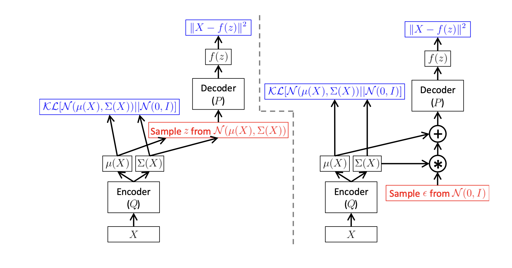
Starting from left-hand side, we are maximizing the log evidence while simultaneously minimizing the distribution regularization term. The right-hand side (ELBO) is similar to auto-encoder, where we map \(X \rightarrow \mathbf{z}\) using \(Q\), then decode back to \(X\) using \(P\).

The right-hand side can be optimized using gradient decent.

Optimize the Objective

How can we optimize the right-hand side (ELBO) ? we first need to be a bit more specific about the form that \(Q(\mathbf{z} | X)\) will take. The usual choice is to say that \(Q(\mathbf{z} | X) = N(\mathbf{z} | \mu(X), \Sigma(X))\), in practice, \(\mu, \Sigma\) are parametrized using NN.

Gaussian Process

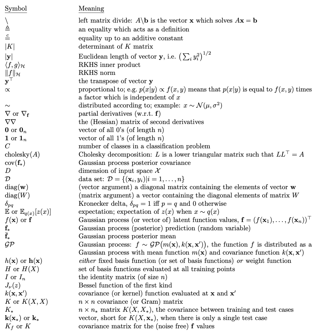
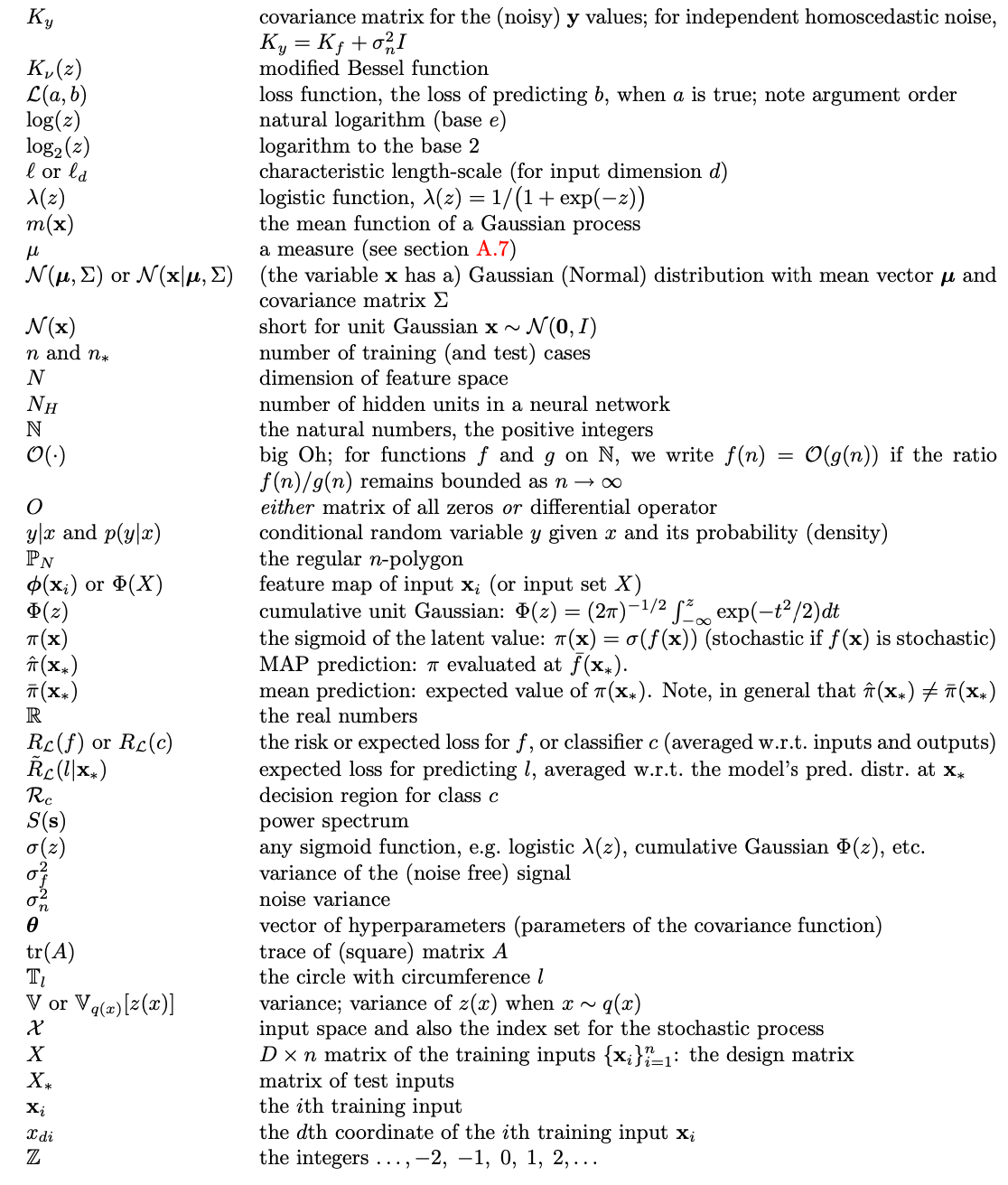
Notations

Gaussian Identities

The multivariate Gaussian distribution has a joint probability density (Bayesian):

\[p(\mathbf{x} | \mathbf{m}, \Sigma) = (2\pi)^{-\frac{D}{2}} |\Sigma|^{-\frac{1}{2}} e^{-\frac{1}{2} (\mathbf{x} - \mathbf{m})^T \Sigma^{-1} (\mathbf{x} - \mathbf{m})}\]

Where \(\mathbf{m}\) is the mean vector of length \(D\) and \(\Sigma\) is the symmetric \(D \times D\), positive definite covariance matrix. As a shorthand, we write \(\mathbf{x} \sim N(\mathbf{m}, \Sigma)\)

Let \(\mathbf{x}, \mathbf{y}\) be jointly Gaussian random vectors:

$$$$

Regression

A Function Space View

Definition 2.1: Gaussian Process

A Gaussian Process is a collection of random variables, any finite number of which have joint Gaussian distribution.

A Gaussian process is completely specified by its mean function and covariance function. We define mean function \(m(\mathbf{x})\) and the covariance function \(k(\mathbf{x}, \mathbf{x}^\prime)\) of a real process \(f(\mathbf{x})\) as:

\[m(\mathbf{x}) = E[f(\mathbf{x})] \quad \quad k(\mathbf{x}, \mathbf{x}^\prime) = E[(f(\mathbf{x}) - m(\mathbf{x}))(f(\mathbf{x}^\prime) - m(\mathbf{x}^\prime))]\]

and given \(N\) examples, we write the Gaussian process \(f := (f(\mathbf{x}_1) , ...., f(\mathbf{x}_N))\) as:

\[f(\mathbf{x}) \sim GP(m(\mathbf{x}), k(\mathbf{x}, \mathbf{x}^\prime))\]

where the random variables represent the value of the function \(f\) at location \(\mathbf{x}\). Often Gaussian process are defined over time, where the index set of the random variables is time. This is not the case in our use of GPs, here the index set \(\mathbb{X}\) is the set of possible inputs. In our case, we identify the random variables s.t \(f_i := f(\mathbf{x}_i)\) corresponding to training example \((\mathbf{x}_i, y_i)\).