MDP

Based on Prof Amir-massoud Farahmand's Lecture on RL

Define our MDP different from Introduction to RL book:

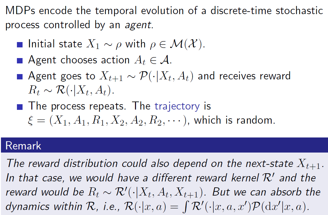
Where \(M(X)\) is the space of all probability distributions defined over the state space X

So a sample of the process can be described as a rollout or trajectory:

\[\tau = X_1, A_1, R_1, X_2, A_2, R_2, ...\]

A deterministic dynamical system always behave exactly the same given the same starting state and action, that is, they can be described as a transition function \(f\) instead of transition distribution \(P\)

\[x_{t+1} = f(x, a)\]

Policy

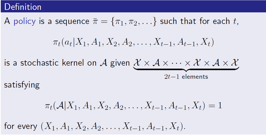
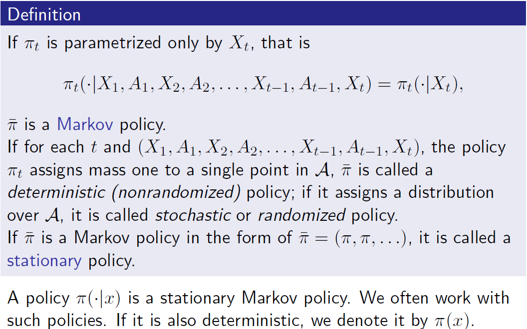
Policy induced Transition Kernels

Rewards and Returns

Let's define expected reward as:

\[r(x, a) = E[R | X=x, A=a]\]

then the expected reward following policy pi is defined as

\[r^{\pi} (x) = E_{a \sim \pi(a | x)} [R | X=x]\]

Define return following policy \(\pi\) as discounted sum of rewards starting from \(X_1\):

\[G^{\pi} = R_1 + \gamma R_2 + ... + \gamma^{T-1} R_{T} = \sum^{\infty}_{k=t} \gamma^{k - t}R_{t}\]

or any starting at any step \(X_{t}\):

\[G^{\pi}_{t} = \sum^{\infty}_{k=t} \gamma^{k - t}R_{t}\]

Note that \(\gamma\) is a part of the problem setting, it is usually not a hyperparameter. One way to think about is as a constant probability of termination of \(1 - \gamma\). Or we can set \(\gamma = 1\) when we have episodic tasks..

Example

Finite horizon example:

• Start at \(X_1 \sim \rho\)
• Select \(A_1 \sim \pi(\cdot | X_1)\)
• Get \(R_1 \sim R(\cdot | A_1, X_1)\)
• Get \(X_2 \sim P(\cdot | A_1, X_1)\)
• ...
• ...
• Get \(R_{T} \sim R(\cdot | X_{T}, A_{T})\)
• Get \(X_{T+1} \sim P(\cdot | X_{T}, A_{T})\) (This is the terminal state, which is often dropped because it has value of 0)

The process stops!

Value functions

Next we can define value functions as:

State value function (alias: Value function, V, v) starting from state x and following policy \(\pi\):

\[V^{\pi}(x) = E[G_1^{\pi} | X_{1} = x] = E[G^{\pi}_{t} | X_{t} = x] \text{ (Markov Property)}\]

Action value function following policy \(\pi\) starting from state x and taking action a:

\[Q^{\pi} (x, a) = E[G_1^{\pi} | X_{1} = x, A_{1} = a] = E[G^{\pi}_{t} | X_{t} = x, A_{t} = a] \text{ (Markov Property)}\]

in the terminal formulation, the value function \(V_{term}^{\pi}\) can be written as:

\[V_{term}^{\pi} = E[R_{1} + R_2 + .... + R_{t + T} | X_1 = x] \;\;\;\;\;\; \forall x \in X\]

The process terminates at time \(t + T\) according to \(\gamma\). In this case the termination should be assumed to always occur in a finite number of steps (ie. if we have episodic task we can set \(\gamma = 1\)).

Another formulation

We can also define the T-step rollout or trajectory distribution \(P(\tau | \pi)\) following policy \(\pi\):

\[P(\tau | \pi) = \rho(X_1)\prod_{t=1}^{T} P(X_{t+1}| X_{t}, A_{t}) \pi(A_t | X_{t}) R(R_t | X_{t}, A_{t})\]

Then:

\[R(\tau) = G^{\pi}_{1} = \sum^{T}_{k=1} \gamma^{k - t}R_{t}\]

\[J(\pi) = E_{\tau \sim P(\tau | \pi) }[R(\tau)] = \int R(\tau) P(d\tau | \pi)\]

\[V^{\pi} (x) = E_{\tau \sim P(\tau | \pi, X_1=x)}[R(\tau) | X_1 = x]\]

And:

\[J(\pi) = \int V^{\pi} (x) d\rho(x)\]