Deterministic Policy Gradient

Deterministic Policy Gradient Algorithms

Introduction

In traditional policy gradient algorithms, policy is parametrized by a probability distribution \(\pi_{\theta} (a | s) = P[a | s; \theta]\) that stochastically selects action \(a\) in state \(s\) according to parameter vector \(\theta\). In this paper, the authors consider deterministic policies \(a = \mu_{\theta} (s)\).

From a practical viewpoint, there is a crucial difference between the stochastic and deterministic policy gradients. In the stochastic case, the policy gradient integrates over both state and action spaces, whereas in the deterministic case it only integrates over the state space:

\[E_{X\sim \rho^{\pi_\theta}A \sim \pi_{\theta}} [\nabla log \pi(A | X) Q^{\pi_{\theta}} (X, A)]\]

Thus, computing deterministic policies may require less samples.

An off-policy learning scheme is introduced here to ensure adequate exploration (i.e The basic idea is to choose actions according to a stochastic behaviour policy).

Notations

Notations are simplified so that the random variables in the conditional density are dropped, and \(\pi_{\theta} = \pi\), the subscripts are dropped for simplicity

Initial state distribution \(p_1(s_1)\), stationary transition dynamics distribution \(p(s_{t+1} | s_{t}, a_{t})\), deterministic reward function \(r(x, a)\). Stochastic policy is represented as \(\pi_{\theta} (a_t | s_t)\). A trajectory of the process is represented as \(h_{1:T} = s_1, a_1, r_1, ...., s_T, a_T\).

The return is the total discounted reward

\[r_t^{\gamma} = \sum^{\infty}_{k = t} \gamma^{k-t} r(s_k, a_k)\]

Value functions:

\[V^{\pi} (s) = E[r_1^{\gamma} | S_1=s; \pi]\]

\[Q^{\pi} (s, a) = E[r_1^{\gamma} | S_1=s, A_1=a; \pi]\]

The objective is to find a policy \(\pi\) that maximize \(J(\pi)\)

\[J(\pi) = E_{s_1 \sim p_1}[r_1^{\gamma} | \pi]\]

Define t step transition probability following \(\pi\) starting from \(s\) as \(p^{\pi}(s \rightarrow s^{\prime}; t)\)

The un-normalized discounted future state distribution:

\[\rho^{\pi} (s^{\prime}) \triangleq \int_s \sum^{\infty}_{t=1} \gamma^{t-1} p(s) p^{\pi}(s \rightarrow s^{\prime}; t) ds\]

The performance objective as expectation:

\[J(\pi) = E_{s \sim \rho^{\pi} (\cdot), a \sim \pi(\cdot | s)} [r(s, a)]\]

Where this expectation is over the un-normalized discounted future state distribution. By replacing discounted future state distribution with stationary state distribution, we have average reward performance measure.

The policy gradient can be written as:

\[\begin{aligned} \nabla_{\theta} J(\pi_\theta) &= \int_S \rho^{\pi} (s) \int_A \nabla_{\theta} \pi_\theta (a | s) Q^{\pi} (s, a) da ds\\ &= E_{s\sim \rho^{\pi} (\cdot), a \sim \pi_{\theta}}[\nabla_{\theta} \log \pi_\theta (a | s) Q^{\pi} (s, a)] \end{aligned}\]

Off-Policy Actor-Critic

It is often useful to estimate the policy gradient off-policy from trajectories sampled from a distinct behaviour policy \(\beta(a | s) \neq \pi_{\theta} (a | s)\). In an off-policy setting, the performance objective is typically modified to be the value function of the target policy averaged over the state distribution of the behaviour policy as initial state.

\[\begin{aligned} J_{\beta} (\pi_{\theta}) &= \int_s \rho^{\beta} (s) V^{\pi} (s) ds\\ &= \int_s \int_a \rho^{\beta} (s) \pi_{\theta} (a | s) Q^{\pi}(s, a) dads\\ \end{aligned}\]

Differentiating the performacne objective and applying an approximation gives the off-policy policy gradient:

\[\begin{aligned} \nabla_{\theta} J_{\beta} (\pi_{\theta}) &\approx \int_s \int_a \rho^{\beta} (s) \nabla_{\theta} \pi_{\theta} (a | s) Q^{\pi}(s, a) dads\\ &= E_{s \sim \rho^\beta, a \sim \beta_{\theta}}[\frac{\pi_{\theta} (a | s)}{\beta (a | s)} \nabla_{\theta} \log \pi_{\theta} (a | s) Q^{\pi} (s, a)]\\ \end{aligned}\]

Gradients of Deterministic Policies

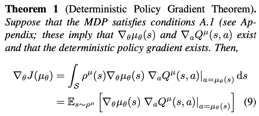
Deterministic Policy Gradient Theorem

Let:

\[J(\mu_{\theta}) = E_{s \sim \rho^{\mu_{\theta}} (\cdot)} [r(s, \mu_{\theta}(s))]\]

Note here that \(\mu_{\theta}\) is the deterministic policy. It is deterministic function of state, and it outputs action (does not represent a probability distribution anymore)

Proof

\[\begin{aligned} \nabla_{\theta} V^{\mu_{\theta}} (s) &= \nabla_{\theta} Q^{\mu_{\theta}} (s, \mu_{\theta} (s))\\ &= \nabla_{\theta} (r(s, \mu_{\theta} (s)) + \int_{s^{\prime}} p(s^{\prime} | s, \mu_{\theta} (s)) V^{\mu_{\theta}} (s^{\prime}) ds^{\prime})\\ &= \nabla_{\theta} \mu_{\theta} (s) \nabla_{a} r(s, a) + \int_{s^{\prime}} \nabla_{\theta} \mu_{\theta} (s) \nabla_{a} p(s^{\prime} | s, a) V^{\mu_{\theta}} (s^{\prime}) ds^{\prime} + \int_{s^{\prime}} p(s^{\prime} | s, \mu_{\theta} (s)) \nabla_{\theta} V^{\mu_{\theta}} (s^{\prime}) ds^{\prime}\\ &= \nabla_{\theta} \mu_{\theta} (s) \nabla_{a} (r(s, a) + \int_{s^{\prime}} p(s^{\prime} | s, a) V^{\mu_{\theta}} (s^{\prime})ds^{\prime}) + \int_{s^{\prime}} p(s^{\prime} | s, \mu_{\theta} (s)) \nabla_{\theta} V^{\mu_{\theta}} (s^{\prime}) ds^{\prime} \\ &= \nabla_{\theta} \mu_{\theta} (s) \nabla_{a} Q^{\mu_{\theta}} (s, a) + \int_{s^{\prime}} p(s^{\prime} | s, \mu_{\theta} (s)) \nabla_{\theta} V^{\mu_{\theta}} (s^{\prime}) ds^{\prime} \end{aligned}\]

Just like Stochastic Policy Gradient Theorem proof, if we keep expanding \(V^{\mu_{\theta}}\), we will end up with:

\[\nabla_{\theta} V^{\mu_{\theta}} (s) = \int_{s^{\prime}} \sum^{\infty}_{t=0} \gamma^{t} p^{\mu_{\theta}}(s \rightarrow s^{\prime}; t) \nabla_{\theta} \mu_{\theta} (s^{\prime}) \nabla_{a} Q^{\mu_{\theta}} (s^{\prime}, a) ds^{\prime}\]

Then our objective can be written as:

\[\begin{aligned} \nabla_{\theta} J(\mu_{\theta}) &= \int_{s_1} p_1(s_1) \nabla_{\theta} V^{\mu_{\theta}} (s_1) ds_1\\ &= \int_{s_1} p_1(s_1) \int_{s^{\prime}} \sum^{\infty}_{t=0} \gamma^{t} p^{\mu_{\theta}}(s_1 \rightarrow s^{\prime}; t) \nabla_{\theta} \mu_{\theta} (s^{\prime}) \nabla_{a} Q^{\mu_{\theta}} (s^{\prime}, a) ds^{\prime} ds_1\\ &= \int_{s^{\prime}} \rho^{\mu_{\theta}} (s^{\prime}) \nabla_{\theta} \mu_{\theta} (s^{\prime}) \nabla_{a} Q^{\mu_{\theta}} (s^{\prime}, a) ds^{\prime}\\ &= E_{s \sim \rho^{\mu_{\theta}} (\cdot)} [\nabla_{\theta} \mu_{\theta} (s) \nabla_{a} Q^{\mu_{\theta}} (s, a) |_{a = \mu_\theta(s)}] \end{aligned}\]

Theorem 2

This theorem shows that the familiar machinery of policy gradient. All PG methods are applicable to deterministic policy gradient.

Off Policy Deterministic Actor-Critic

The performance objective is:

\[J_{\beta}(\mu_{\theta}) = E_{s \sim \rho^{\beta} (\cdot)} [r(s, \mu_{\theta}(s))]\]

The gradient:

\[\begin{aligned} \nabla_{\theta} J_{\beta} (\pi_{\theta}) &\approx \int_s \rho^{\beta} (s) \nabla_{\theta} \mu_{\theta} (s) \nabla_{a} Q^{\mu_{\theta}} (s, a) |_{a = \mu_\theta(s)} ds\\ &= E_{s \sim \rho^\beta}[\nabla_{\theta} \mu_{\theta} (s) \nabla_{a} Q^{\mu_{\theta}} (s, a) |_{a = \mu_\theta(s)} ]\\ \end{aligned}\]

This equation gives the off-policy deterministic policy gradient. We now develop an actor-critic algorithm that updates the policy in the direction of the off-policy deterministic policy gradient. We can see that the integral over \(a\) is removed because we are using the deterministic policy, that is, we can avoid importance sampling in the critic.

We substitute a differentiable action-value function \(Q^{w} (s, a)\) in place of the true action-value function \(Q^{\mu} (s, a)\). A critic estimates the action-value function \(Q^{w} (s, a) \approx Q^{\mu} (s, a)\). In the below off-policy deterministic actor critic algorithm, the critic estimates the action-value function using the samples from \(\rho^\beta\)

Compatible Function Approximation

Compatible Function Approximator in Stochastic Case

In general, substituting an approximate \(Q^{w} (s, a)\) will not necessarily follow the true gradient. Similar to the stochastic ase, only compatible function approximators are guaranteed to be unbiased. Recall that a function approximator \(f_w\) is compatiable if:

1. \(f_w\) is found by minimizing the square loss \(E_{s \sim \rho^{\pi_{\theta}}, a \sim \pi_{\theta}} [(Q^{\pi} (s, a) - f_{w} (s, a))^2]\)
2. \(\nabla_{w} f_w (s, a) = \nabla_{\theta} \pi_{\theta}(s, a) \frac{1}{\pi(s, a)}\), this is satisfied only when \(f_w (s, a) = \nabla_{\theta} \log \pi_{\theta}(s, a) w^T\)

These conditions imply:

\[\nabla_{\theta} J(\pi_\theta) = E_{s\sim \rho^{\pi} (\cdot), a \sim \pi_{\theta}}[\nabla_{\theta} \log \pi_\theta (a | s) f_w(s, a)]\]

Proof

Notice that, at the fixed point, we will have:

\[Q^{\pi} (s, a) - f_w (s, a) = 0\]

and the gradient of the loss:

\[\nabla_{w} E_{s \sim \rho^{\pi_{\theta}}, a \sim \pi_{\theta}} [(Q^{\pi} (s, a) - f_{w} (s, a))^2] = E_{s \sim \rho^{\pi_{\theta}}, a \sim \pi_{\theta}} [(Q^{\pi} (s, a) - f_{w} (s, a)) \nabla_{w} f_{w} (s, a)] = 0\]

By substitute condition 2 into the above equation, we have:

\[E_{s \sim \rho^{\pi_{\theta}}, a \sim \pi_{\theta}} [(Q^{\pi} (s, a) - f_{w} (s, a)) \nabla_{\theta} \log \pi_{\theta}(s, a)] = 0\]

Since the gradient of loss is 0, we can subtract it from the policy gradient:

\[\begin{aligned} \nabla_{\theta} J(\pi_\theta) &= E_{s \sim \rho^{\pi_{\theta}}, a \sim \pi_{\theta}} [\nabla_{\theta} \log \pi_\theta (a | s) Q^{\pi} (s, a)] - E_{s \sim \rho^{\pi_{\theta}}, a \sim \pi_{\theta}} [(Q^{\pi} (s, a) - f_{w} (s, a)) \nabla_{\theta} \log \pi_{\theta}(s, a)]\\ &= E_{s\sim \rho^{\pi} (\cdot), a \sim \pi_{\theta}}[\nabla_{\theta} \log \pi_\theta (a | s) f_w(s, a)] \end{aligned}\]

Compatible Function Approximator in Deterministic Case

Similar in above stochastic case, we want to find a class of compatible function approximators \(Q^{w} (s, a)\) such that the gradient is preserved. In order words:

\[\nabla_a Q^{w} (s, a) = \nabla_a Q^{\mu_{\theta}} (s, a)\]

So that we could replace \(\nabla_a Q^{\mu_{\theta}} (s, a)\) with \(\nabla_a Q^{w} (s, a)\) and still have the true gradient preserved.

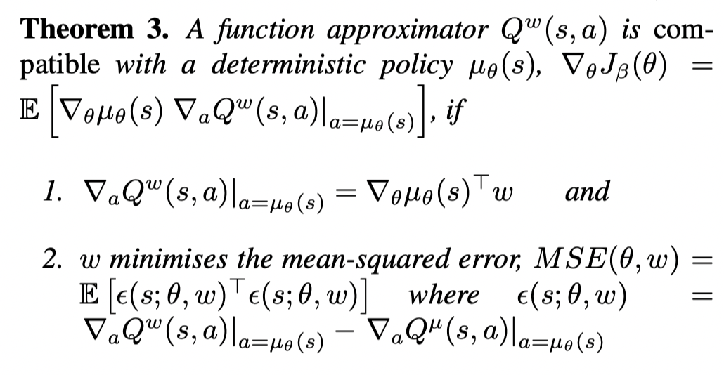
This theorem applies to both on-policy and off-policy cases

Proof

The proof basically follows the stochastic case:

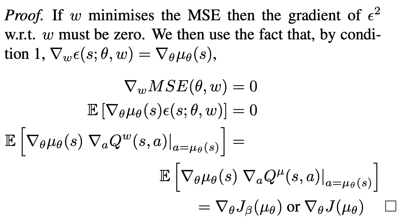
So for any deterministic policy \(\mu_\theta (s)\), there always exists a compatible function approximator of the form:

\[f_{w} (s, a) = \phi(s, a)^T \nabla_{\theta} \mu_{\theta} (s)^Tw + V^{v} (s)\]

Where \(V^{v} (s)\) can be any baseline function that is independent of the action \(a\) and \(\nabla_{a} \phi(s, a)^T = 1\). This function satisfies condition 1. However, in order to satisfy condition 2, we need to find the parameters \(w\) that minimize the mse between th gradient of \(Q^w\) and the true gradient. Since, acquiring unbiased samples of the true gradient is difficult, in practice, we learn \(w\) using a standard policy evaluation method that does not exactly satisfy condition 2 (ie. using SARSA, Q-learning through semi-gradient TD).

We denote the reasonable solution to the policy evaluation problem by \(Q^{w} (s, a) \approx Q^{\mu} (s, a)\) and will therefore approximately satisfy

\[\nabla_a Q^{w} (s, a) \approx \nabla_a Q^{\mu_{\theta}} (s, a)\]

Compatible Off-Policy Deterministic Actor-Critic Algorithm (COPDAC)

The Compatible off-policy deterministic actor-critic algorithm consists of two compoenents:

1. The critic is a linear function approximator that estimates the action-value from features:

   \[a \nabla_{\theta}\mu_{\theta} (s)^Tw + V^{v} (s)\]

   This can be learnt off-policy using samples of a behaviour policy \(\beta(a | s)\), for example using Q-learning or gradient Q-learning. \(V^{v} (s)\) is parametrized linearly as \({\phi(s)}^T v\).

2. The actor then updates its parameters in the direction of the critic's action-value gradient.

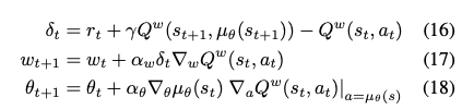
The following COPDAC-Q algorithm uses a simple Q-learning critic:

1. Calculate the TD error for semi gradient TD update

   \[\delta_t = r_t + \gamma Q^{w} (s_{t+1}, \mu_{\theta}(s_{t+1})) - Q^{w} (s_t, a_t)\]

2. Update \(V^{v} (s)\)

   \[v_{t + 1} = v_t + \alpha_v \delta_t \phi(s_t)\]

3. Update \(Q^{w} (s, a)\)

   \[w_{t + 1} = w_t + \alpha_w \delta_t a_t^T \nabla_{\theta}\mu_{\theta} (s_t)\]

4. Update the actor \(\mu_{\theta} (s)\):

   \[\theta_{t + 1} = \theta_{t} + \alpha_{\theta} \nabla_{\theta}\mu_{\theta} (s_t) (\nabla_{\theta}\mu_{\theta}^T (s_t) w_t)\]