Probability (1)
Probability Background (1)
Sets
A set is a collection of objects, which are the elements of set. If S is a set and \(x\) is an element of \(S\), we write \(x \in S\). If \(x\) is not an element of \(S\), we write \(x \notin S\). A set can have no elements, in which case it is called the empty set, denoted by \(\emptyset\).
Finite, Countable, Uncountable
If \(S\) contains a finite number of elements, say \(x_1, x_2, ..., x_n\), we write it as list of the elements in braces:
\[S = \{x_1, x_2, ...., x_n\}\]
if \(S\) contains countable infinitely many elements \(x_1, x_2, ...\), we can write:
\[S = \{x_1, x_2, ... \}\]
\(S\) is countable infinite, if the set is countable but has infinitely many elements. However, a set with uncountable elements can not be written down in a list.
We can denote set of all \(x\) that have certain property \(P\):
\[\{x | x \text{ satisfies } P\}\]
ie. the set of even integers can be written as \(\{k | k/2 \text{ is integer}\}\), \(\{x | 0 \leq x \leq 1\}\) (uncountable)
Subsets and Universal set
If every element of a set \(S\) is also an element of a set \(T\), then \(S\) is a subset of \(T\), we denote as \(S \subset T\) or \(T \subset S\). If \(S \subset T\) and \(T \subset S\), the two sets are equal. We also denote universal set to be \(\Omega\) which contains all objects that could conceivably be of interest in a particular context.
Set Functions
Many of the functions used in calculus are functions that map real numbers into real numbers. We are concerned also with functions that map sets into real numbers. Such functions are naturally called functions of a set or more simply set functions. They are usually used to measure subsets of a given set.
Examples:
Let \(C=\mathbf{R}\), the set of real numbers. For a subset \(A \in C\), let \(Q(A)\) be equal to the number of points in \(A\) that correspond to positive integers. Then \(Q(A)\) is a set function of the set \(A\). Thus, if \(A = \{x: 0 < x < 5\} \implies Q(A) = 4\)
Often our set functions are defined in terms of sums or integrals, the symbol:
\[\int_A f(x) dx\]
means the ordinary integral of \(f(x)\) over a prescribed one-dimensional set \(A\), and the symbol
\[\underset{A}{\int\int} g(x, y) dx dy\]
means the integral of \(g(x, y)\) over a prescribed two-dimensional set \(A\).
Examples:
Let \(C\) be the set of all nonnegative integers and let \(A\) be a subset of \(C\). Define the set function \(Q\) by \[Q(A) = \sum_{n \in A} 3^{n}\]
Let \(C\) be the interval of positive real numbers, \(C = (0, \infty)\). Let \(A\) be a subset of \(C\). Define the set function \(Q\) by \[Q(A = \int_{A} e^{-x} dx\] \[Q((1, 3)) = \int^{3}_{1} e^{-x} dx\] \[Q(C) = \int^{\infty}_{0} e^{-x} dx = 1\]
Probability Models
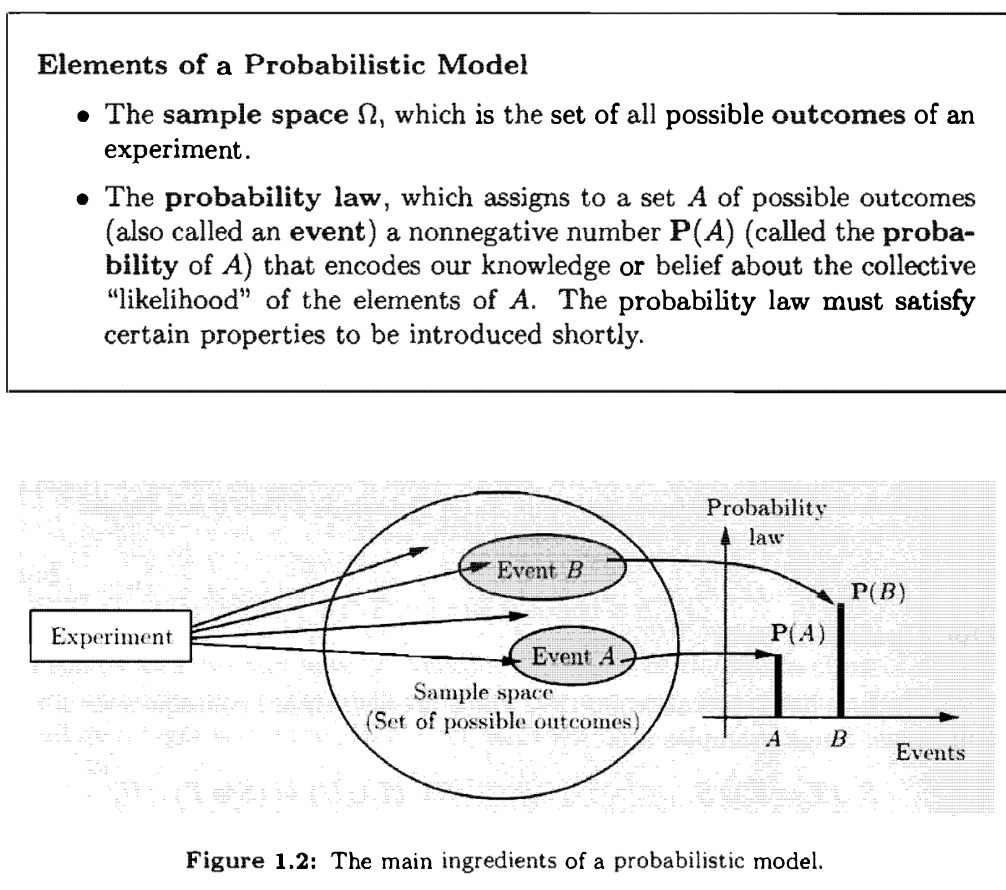
A probabilistic model is a mathematical description of an uncertain situation.
Sample Spaces and Events
Every probabilistic model involves an underlying process, called the experiment, that will produce exactly one out of several possible outcomes. The set of all possible outcomes is called the sample space of the experiment, and is denoted by \(\Omega\) (Universal Set). A subset of the sample space, that is, a collection of possible outcomes, is called an event. Any collection of possible outcomes, including the entire sample space \(\Omega\) and its complement the empty set. There is no restriction on what constitutes an experiment. (ie. it can be one toss of the coin, three tosses of coin, or an infinite sequence of tosses). However, in this formulation, there is only one experiment (three tosses is one experiment rather than three experiments).
The sample space of an experiment may consist of a finite, or an infinite number of possible outcomes.
Regardless of their number. different elements of the sample space should be distinct and mutually exclusive, so that when the experiment is carried out there is a unique outcome. For example, the sample space associated with the roll of a die cannot contain "1 or 3" as a possible outcome and also "1 or 4" as another possible outcome. If it did, we would not be able to assign a unique outcome when the roll is a 1.
A given physical situation may be modeled in several ways, depending pending on the kind of questions that we are interested in . Generally, the sample space chosen for a probabilistic model must be collectively exhaustive, in the sense that no matter what happens in the experiment, we always obtain an outcome that has been included in the sample space. In addition, the sample space should have enough detail to distinguish between all outcomes of interest to the modeler, while avoiding irrelevant details.
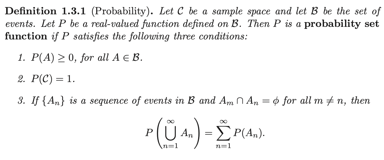
Probability Laws and Probability Set Function
Given an experiment, let \(C\) denotes the sample space of all possible outcomes. We assume that in all cases:
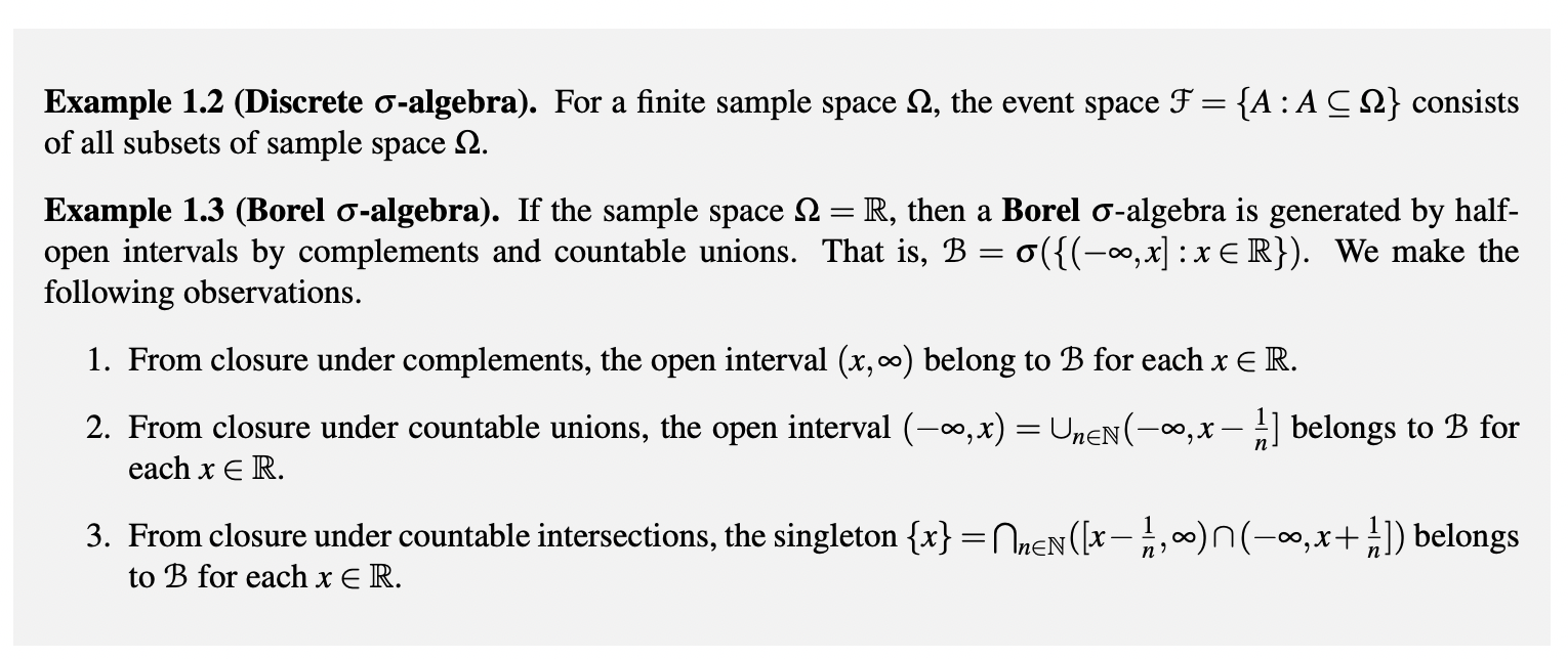
- The collection of events is sufficiently rich to include all possible events of interest.
- The collection is closed under complements and countable unions of these events.
- The collection is closed under countable intersections.
Technically, such a collection of events \(\mathbb{B}\) is called a \(\sigma-\)field of subsets.
In order to visualize a probability law. Consider a unit of mass which is spread over the sample space. Then, \(P(A)\) is simply the total mass that was assigned collectively to the elements of A. For example, \(\Omega = {1, 2, 3, 4, 5, 6}, A = {1, 2}\), \(P(A) = \frac{1}{3}\)
A collection of events whose members are pairwise disjoint, is said to be a mutually exclusive collection and its union is often referred to as a disjoint union. The collection is further said to be exhaustive if the union of its events is the sample space. in which case \(\sum^{\infty}_{n=1} P(A_n) = 1\). We often say that a mutually exclusive and exhaustive collection of events forms a partition of the sample space \(C\).
The probability set function \(P: \mathbb{B} \rightarrow \mathbb{R}\) tells us how the probability is distributed over the set of events, \(\mathbb{B}\). In this sense, we speak of a distribution of probability. We often drop the word set and refer to \(P\) as the probability function.
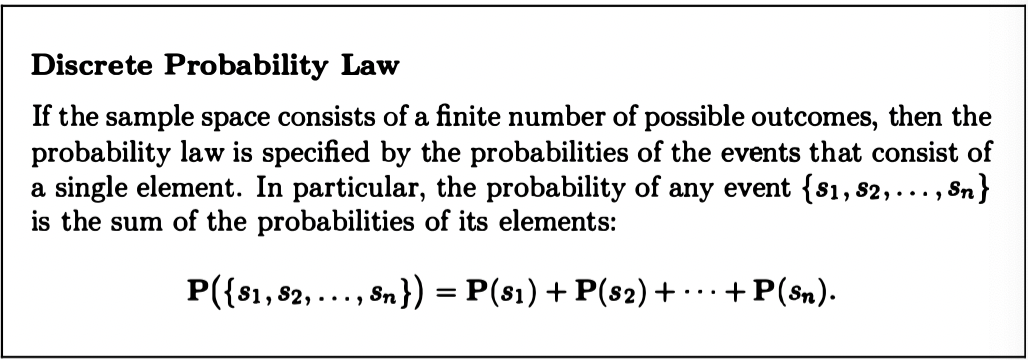
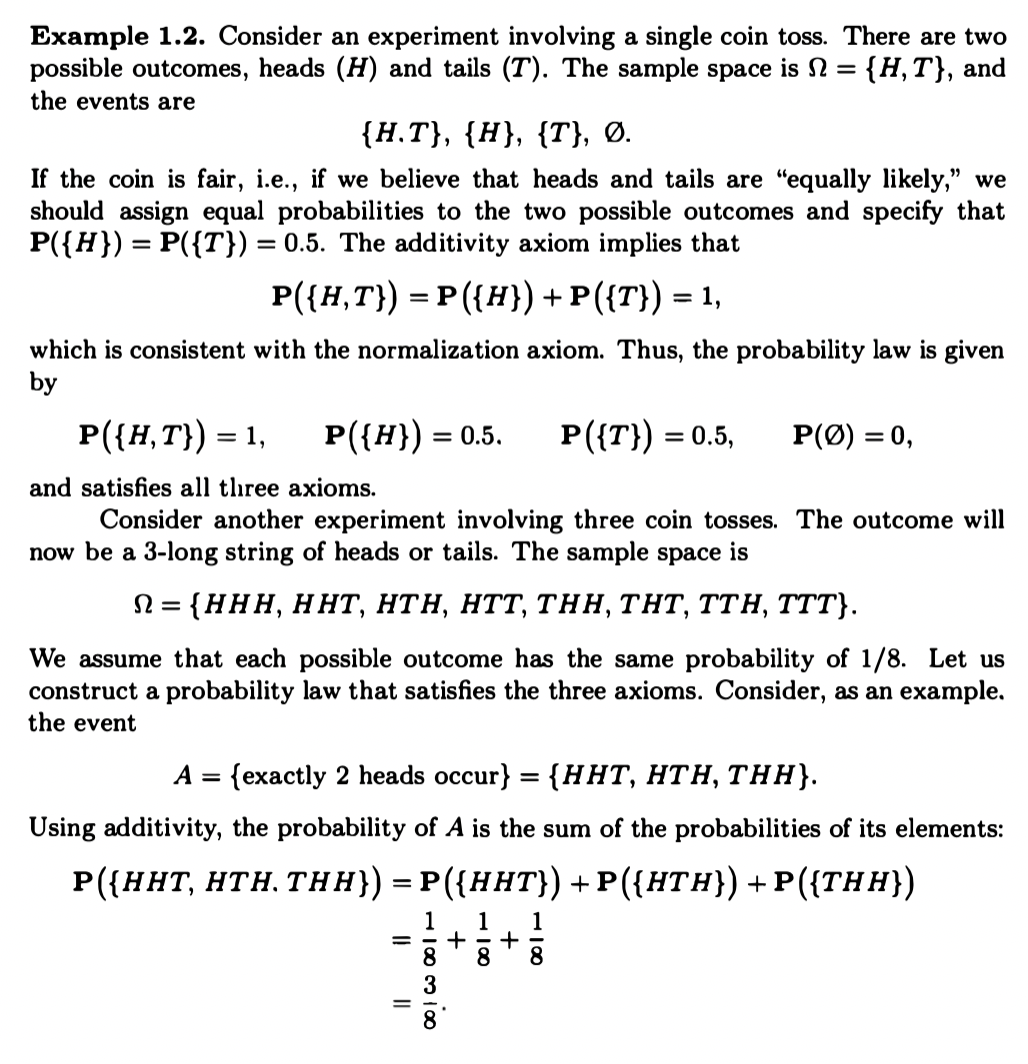
Discrete Model
Additional Properties of Probability
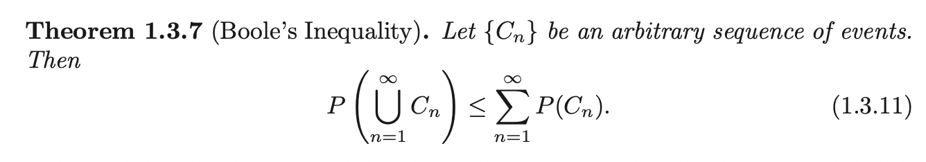
The Inclusion Exclusion Formula:
\[P(C_1 \cup C_2 \cup C_3) = p_1 - p_2 + p_3\]
Where:
\[p_1 = P(C_1) + P(C_2) + P(C_3)\]
\[p_2 = P(C_1 \cap C_2) + P(C_1 \cap C_3) + P(C_2 \bigcap C_3)\]
\[p_3 = P(C_1 \cap C_2 \cap C_3)\]
The Bonferroni's inequality:
\[P(C_1 \cap C_2) \geq P(C_1) + P(C_2) - 1\]
Conditional Probability
In some random experiment, we are interested only in those outcomes that are elements of a subset \(A\) of the sample space \(C\). This means, for our purposes, that the sample space is effectively the subset \(A\).
Let the probability set function \(P(A)\) be defined on the sample space \(C\) and let \(A\) be a subset of \(C\) such that \(P(A > 0)\). We only take those outcomes of the random experiment that are elements of \(A\) to be the sample space. Let \(B\) be another subset of \(C\). The conditional probability of event \(B\) given \(A\) is denoted by the symbol \(P(B | A)\) .
Since \(A\) is now the sample space, the only elements of \(B\) that concern us are those that are also elements of \(A\), that is the elements of \(A \cap B\) and \(A\), relative to the space \(A\), be the same as the ratio of the probabilities of these events relative to the space \(C\), that is, we should have:
\[P(A | A) = 1 \;\;\;\;\;\; P(A \cap B | A) = P(B | A)\]
Moreover, it would seem logically inconsistent if we did not require that the ratio of the probabilities of the events \(A \cap B\) and \(A\), relative to the space \(A\), be the same as the ratio of the probabilities of these events relative to the space \(C\) (ie. if \(P(A) = 0.5, P(B) = 0.2, P(A \cap B) = 0.1, P(A) / P(C) = 1 / 2, P(A \cap B | A) = 0.2\)), that is, we should have:
\[\frac{P(A \cap B | A) }{P(A | A)} = \frac{P(A \cap B)}{P(A)}\]
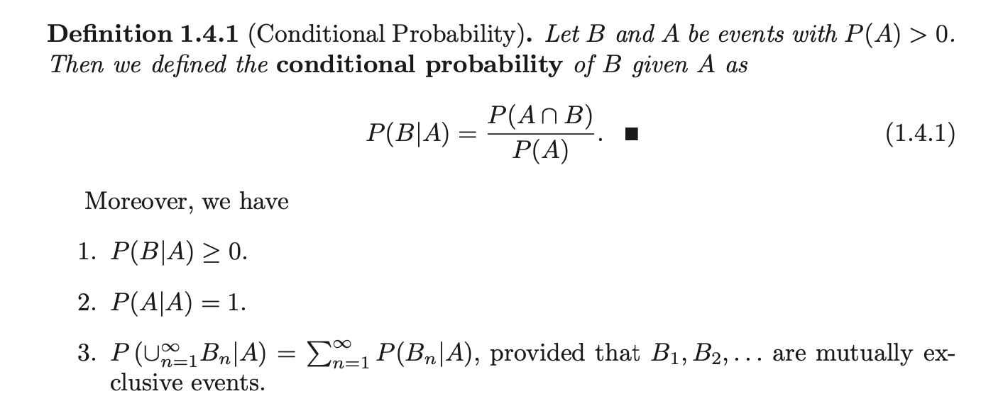
\(P(B|A)\) the conditional probability set function, defined for subsets of \(A\).
Conditional probability provides us with a way to reason about the outcome of an experiment, based on partial information. In more precise terms, given an experiment, a corresponding sample space, and a probability law, suppose that we know that the outcome is within some given event \(B\). We wish to quantify the likelihood that the outcome also belongs to some other given event \(A\). This concept specifies the conditional probability of \(A\) given \(B\), denoted by \(P(A | B)\).
Furthermore, for a fixed event \(B\), it can be verified that the conditional probabilities \(P(A | B), \forall A\) form a legitimate probability law that satisfies the requirements.
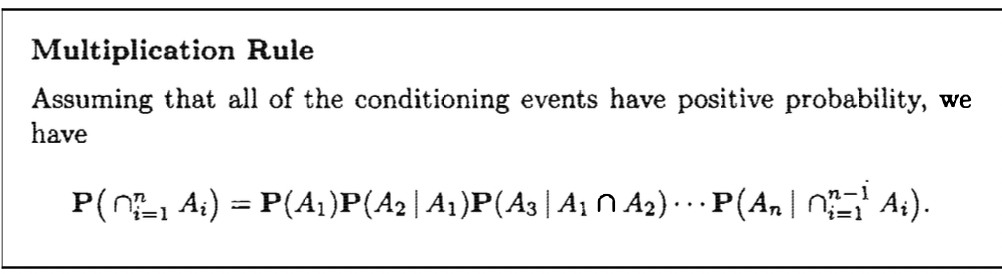
Chain Rule
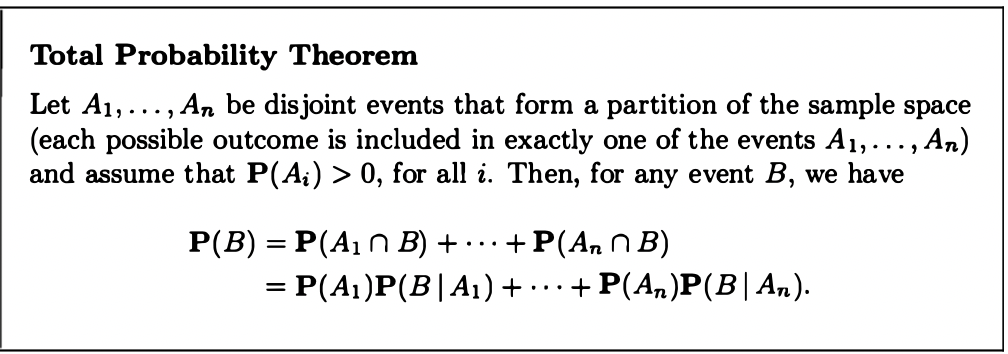
Law of Total Probability
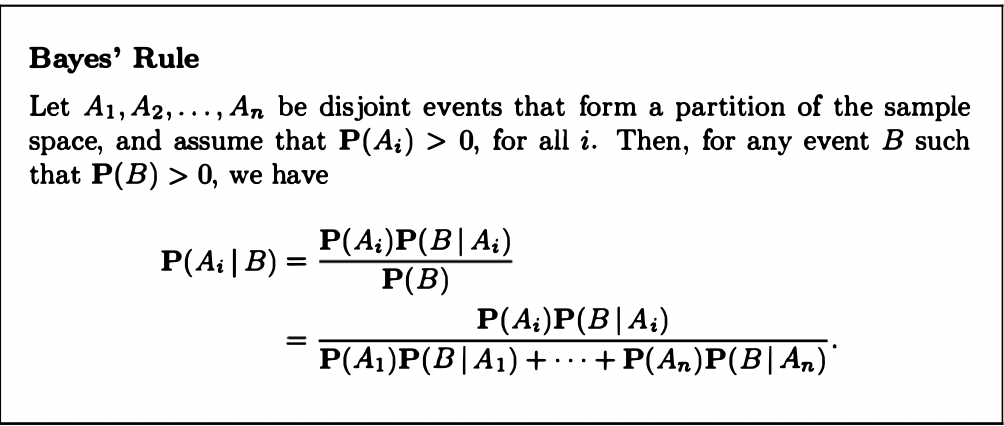
Bayes' Rule
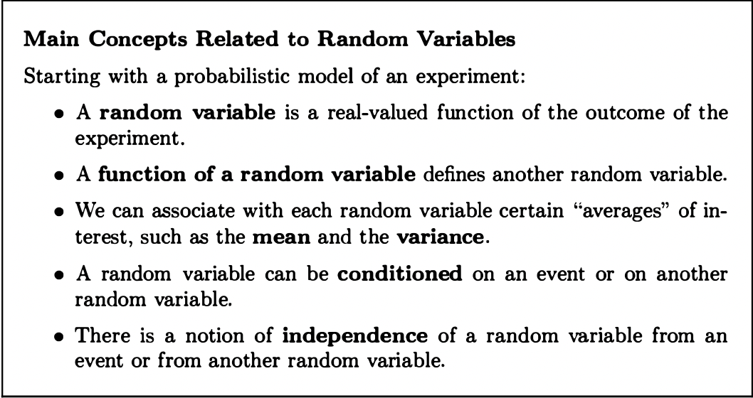
Random Variables
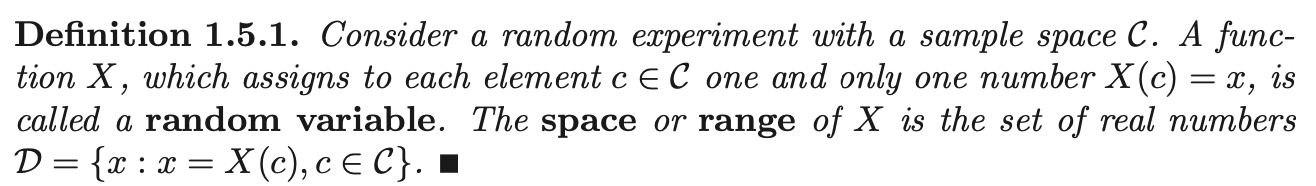
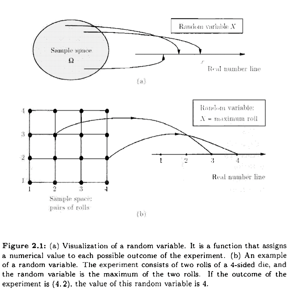
Given an experiment and the corresponding set of possible outcomes (the sample space), a random variable is a real-valued function (max, min etc.) of experiment outcome that associates a particular number with each outcome. We refer to this number as the numerical value or simply the value of the random variable.
Distribution of Random Variable
Given a random variable \(X\), its range \(\mathbb{D}\) becomes the sample space of interest. Besides, inducing the sample space \(\mathbb{D}\), \(X\) also induces a probability which we call the distribution of \(X\).
Assume \(X\) is a discrete random variable with a finite space \(\mathbb{D} = \{d_1, ...., d_m\}\). Define the function \(p_{X} (d_i)\) on \(\mathbb{D}\) by:
\[p_X(d_i) = P[\{c: X(c) = d_i\}], \quad \quad \forall i=1, .... ,m\]
Which is the probability of event that contains the outcomes with value \(X(c) = d_i\), this is called the probability mass function of \(X\). Then the induced probability distribution, \(P_X (\cdot): D \rightarrow \mathbb{R}\), of \(X\) is:
\[P_X (D) = \sum_{d_i \in D} p_X (d_i), \quad \quad D \subset \mathbb{D}\]
Similar to \(P\) which is defined on \(\mathbb{B}\). This \(P_X (\cdot)\) is basically the probability distribution of events defined on sets \(D\), \(P_X (D)\) is the probability of event \(D\) defined on \(\mathbb{D}\).
Cumulative Distribution Function
The pmf of discrete random variable and the pdf of a continuous random variable are quite different entities. The distribution function, though, uniquely determines the probability distribution of a random variable:
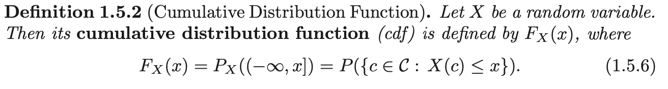
Note that, cdf is defined \(\quad \forall x \in \mathbb{R}\).
Remember that \(P_X (\cdot)\) is the probability set function (distribution) of the random variable \(X\). The cdf is the probability of event (subset of \(\mathbb{D}\), the random variable range space): \(\{a: a \leq x, a \in \mathbb{D}\}\), this is the same as the event (defined on sample space): \(\{c: X(c) \leq x, c \in \mathbb{B}\}\).
Equal in Distribution
Let \(X, Y\) be two random variables. We say that \(X\) and \(Y\) are equal in distribution and write:
\[X \overset{D}{=} Y\]
IFF:
\[F_X(x) = F_Y (x), \quad \quad \quad \forall x \in \mathbb{R}\]
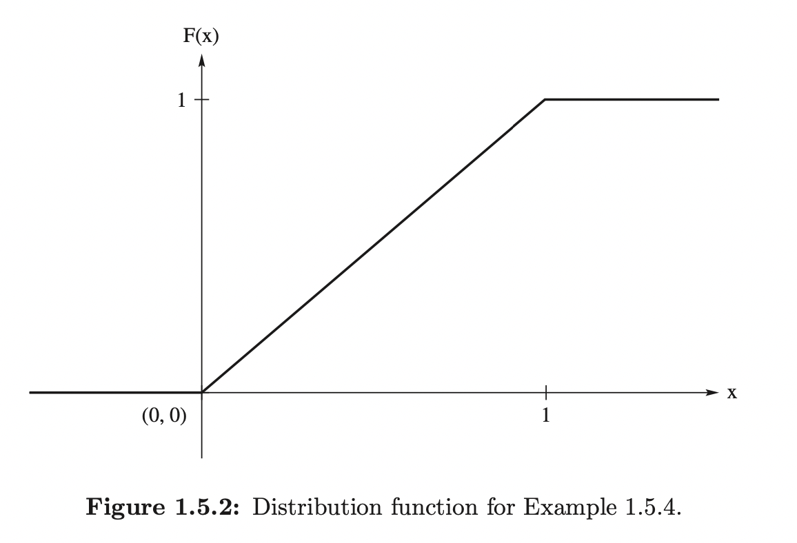
Notice that, equal in distribution does not mean the random variables are the same. For examples, let \(X\) be a random variable sampled from range \([0, 1)\), let \(Y = 1 - X\), then \(Y\) also has range \([0, 1)\). At the same time, for \(x < 0\), the cdf for both random variables is 0, for \(x < 0\), the cdf for both random variables is 1. And, for \(0 \leq x < 1\), the cdf is \(x\) for both random variables. But this two random variables are clearly different.
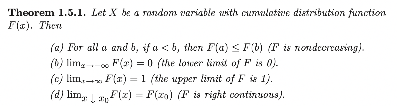
Theorems for CDF
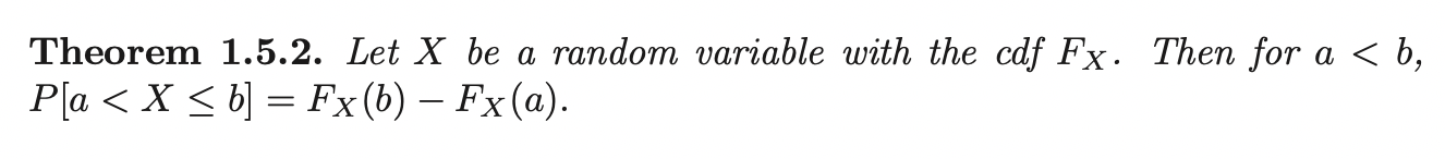
Proof of Theorem 1.5.2
Note that the event \(\{-\infty < X \leq b\} = \{-\infty < X \leq a\} \cup \{a < X \leq b\}\), Then \(\{-\infty < X \leq a\} \cup \{a < X \leq b\}\) are disjoint events, which means:
\[P_X(\{-\infty < X \leq a\} \cup \{a < X \leq b\}) = P_X(\{-\infty < X \leq a\}) + P_X(\{a < X \leq b\})\]
Then,
\[\begin{aligned} P(\{-\infty < X \leq b\}) &= P_X(\{-\infty < X \leq a\}) + P_X(\{a < X \leq b\})\\ \implies F_X (b) &= F_X(a) + P_X(\{a < X \leq b\})\\ \end{aligned}\]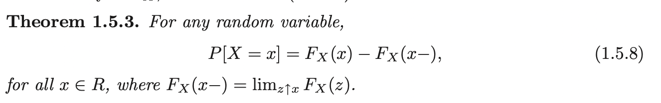
This basically means that the discontinuities of a cdf have mass. That is, if \(x\) is a point of discontinuity of \(F_x\), then we have \(P(X=x) > 0\).
Example:
Let \(X\) have discontinuous cdf: \[ F_X(x)= \begin{cases} 0, \quad &x < 0\\ \frac{x}{2}, \quad &0 \leq x < 1\\ 1, \quad &1 \leq x \end{cases} \] Then: \[P(X=1) = F_X (1) - F_X(1 - ) = 1 - \frac{1}{2} = \frac{1}{2}\]
Discrete Random Variables

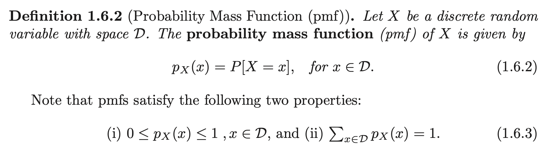
If a function satisfies properties 1, 2 of the pmf, then this function \(p_X\) uniquely determines the distribution (probability set function) of a random variable \(P_X\).
Support
Let \(X\) be a discrete random variable with space \(\mathbb{D}\). We define the support of a discrete random variable \(X\) to be the points in the space (range) of \(X\) which have positive probability. We often denote \(S\) as the support of \(X\). Note that \(S \in \mathbb{D}\), but it may be that \(S = \mathbb{D}\).
If \(x \in S\), then \(p_X (x)\) is equal to the size of the discontinuity of \(F_X\) at \(x\). If \(x \neq S\) then \(P[X=x] = 0\) and hence, \(F_X\) is continues at this \(x\).
Transformations
If we have a random variable \(X\) and we know its distribution (\(P_X, p_X\)). We are interested, though, in a random variable \(Y\) which is some transformation of \(X\) say \(g(X) = Y\). In particular, we want to determine the distribution of \(Y\). Assume \(X\) is discrete with space \(\mathbb{D}_X\). Then the space of \(Y\) is \(D_Y = {g(x): x \in \mathbb{D}_X}\). We consider two case of \(g\):
If \(g\) is one to one. Then, clearly, the pmf of \(Y\) is:
\[p_Y (y) = P_Y(Y = y) = P_X(g(X) = y) = p_X (X = g^{-1} (y)) = p_X (g^{-1} (y))\]
If \(g\) is not one to one. We basically infer the pmf of \(Y\) in a straight forward manner: For each value of \(Y=y\), we infer it:
\[P_X(\{x: g(x) = y, x \in \mathbb{D}\})\]
Example (case 1):
Let X have the pmf: \[ p_X(x)= \begin{cases} \frac{3!}{x!(3 - x)!} {\frac{2}{3}}^x {\frac{1}{3}}^{3 - x}, \quad &x = 0, 1, 2, 3\\ 0, \quad &\text{o. w}\\ \end{cases} \] If \(Y = 2X\), then this is a one to one mapping and \(\frac{1}{2} Y = X\), the pmf of \(Y\): \[p_Y (y) = p_X (\frac{1}{2} y)\] That is: \[ p_Y(y)= \begin{cases} \frac{3!}{(\frac{1}{2} y)!(3 - \frac{1}{2} y)!} {\frac{2}{3}}^x {\frac{1}{3}}^{3 - \frac{1}{2} y}, \quad &y = 0, \frac{1}{2}, 1, \frac{3}{2}\\ 0, \quad &\text{o. w}\\ \end{cases} \]
Example (case 2):
If \(Y = X^2\), for \(\mathbb{D_X} = \{-1, 1\}\). Then the pmf of \(Y\): \[ p_Y(y)= \begin{cases} P_X (\{-1, 1\}) = \underset{x \in \{-1, 1\}}{\sum} p_X (x), \quad &y = 1\\ 0, \quad &\text{o. w}\\ \end{cases} \]
Continuous Random Variables
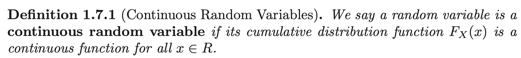
Recall that, a point of discontinuity in cdf has \(P(X=x) = F_X(x) - F_X (x -) > 0\), for any random variable. Hence, for a continuous random variable \(X\), there are no points of discrete mass \(\implies P(X=x) =0, \quad \forall x \in \mathbb{R}\). Most continuous random variables are absolutely continuous:
\[F_X (x) = \int^{x}_{-\infty} f_X(t) dt\]
For some function \(f_X\) or \(f_X (t)\). The function \(f_X (t)\) is called a probabability density function (pdf) of \(X\). If \(f_X (x)\) is also continuous, then the fundamental theorem of calculus implies that:
\[\frac{d}{dx}F_X (x) = \frac{d}{dx}\int^{x}_{-\infty} f_X(t) dt = f_X (x)\]
The support \(S\) of a continuous random variable \(X\) consists of all points \(x\) such that \(f_X(x) > 0\).
If \(X\) is a continuous random variable, then probabilities can be obtained by integration:
\[P_X (a < X \leq b) = F_{X} (b) - F_{X} (a) = \int^{b}_{-\infty} f_X(t) dt - \int^{a}_{-\infty} f_X(t) dt = \int^{b}_{a} f_X(t) dt\]
Also, for continuous random variables:
\[P_X(a < X \leq b) = P_X(a \leq X \leq b) = P_X (a \leq X < b) = P_X(a < X < b)\]
The pdfs satisfy two properties:
\[f_X(x) \geq 0 \quad \quad \quad \int^{\infty}_{-\infty} f_X(t) dt = 1\]
At the same time, if a function satisfies the above two properties then it is a pdf for a continuous random variable.
Quantiles
Quantile (percentiles) are easily interpretable characteristics of a distribution.
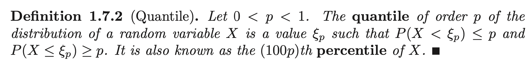
Median is the quantile \(\xi_{\frac{1}{2}}\). It is a point in the domain of \(X\) that divides the mass of the pdf into its lower and upper halves. The first and third quartiles divide each of these halves into quarters. They are respectively \(\xi_{\frac{1}{4}}, \xi_{\frac{3}{4}}\). We label them \(q_1, \; q_2, \; q_3\) respectvely. The difference \(iqr = q_3 - q_1\) is called the inter-quartile range of \(X\).
The median is often used as a measure of center of the distribution of \(X\) (\(P_X\)), while the interquartile range is used as a measure of spread and dispersion of the distribution of \(X\).
Quantiles need not be unique even for continuous random variables with pdfs.
Example:
Any point in the interval (2, 3) serves as a median for the following pdf \[ f(x)= \begin{cases} 3(1 - x)(x - 2), \quad &1 < x < 2\\ 3(3 - x)(x - 4), \quad &3 < x < 4\\ 0, \quad & o. w\ \end{cases} \]
If, however, a quantile, say \(\xi\) is in the support of an absolutely continuous random variable \(X\) with cdf \(F_X(x)\) then \(\xi\) is unique solution to the equation:
\[P_X (X < \xi) = p \implies F_X (\xi) = p \implies \xi = F^{-1}_X (p)\]
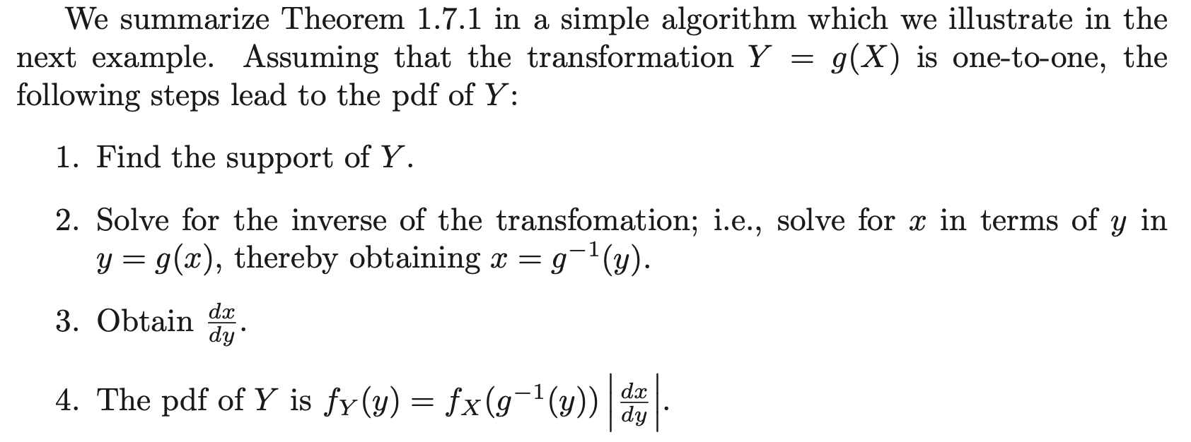
Transformations
Let \(X\) be a continuous random variable with pdf \(f_X\). Let \(Y = g(X)\) be some transformation of \(X\). We can obtain the pdf of \(Y\) by first obtain its cdf.
Example:
\[ F_X(x)= \begin{cases} 0, \quad &x < 0\\ x^2, \quad &0 \leq x < 1\\ 1, \quad & 1 \leq x \end{cases} \] Let \(Y = X^2\) and let \(y\) be in the support of \(Y\), that is \(0< f_Y(y) \implies 0 < y < 1\) (If \(y = 1 \implies f_Y (y) = 0\)). \[F_Y(y) = P_Y (Y < y) = P_X (X < \sqrt{y}) = F_X (\sqrt{y}), \quad \forall 0 < y < 1\] \[\implies F_Y(y) = F_X (\sqrt(y)) = y, \quad \forall 0 < y < 1\] \[ \implies f_Y(y)= \begin{cases} 1, \quad &0 < y < 1\\ 0, \quad &o.w \end{cases} \]
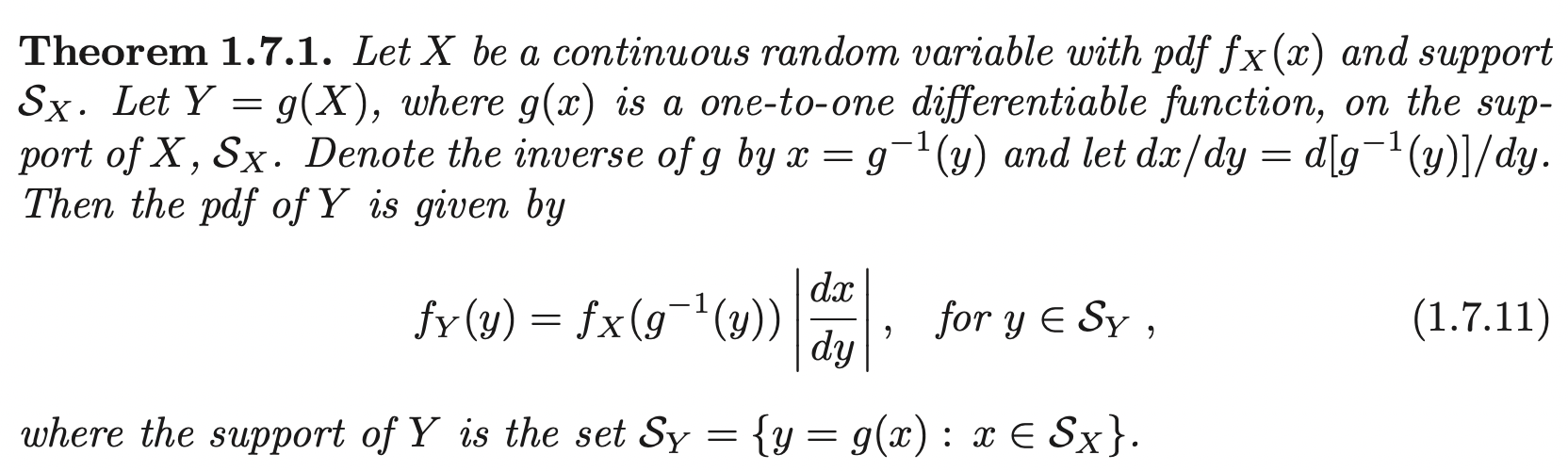
Proof:
\[F_Y(y) = P(X < g^{-1} (y) = F_X (g^{-1} (y)) \implies \frac{d}{dy} F_Y(y) = \frac{d}{dy} F_X (g^{-1} (y)) = f_X (g^{-1} y) |\frac{d}{dy} g^{-1} (y)|\]
In this case, we refer \(\frac{d}{dy} g^{-1} (y)\) as the Jacobian of the inverse transformation.
Expectation
When dealing with R.V that takes a countably infinite number of values, one has to deal with the possibility that the infinite sum \(\sum_x xp_X(x)\) is not well-defined. More concretely, the expectation is well-defined if
\[\sum_x |x| p_X(x) < \infty\]
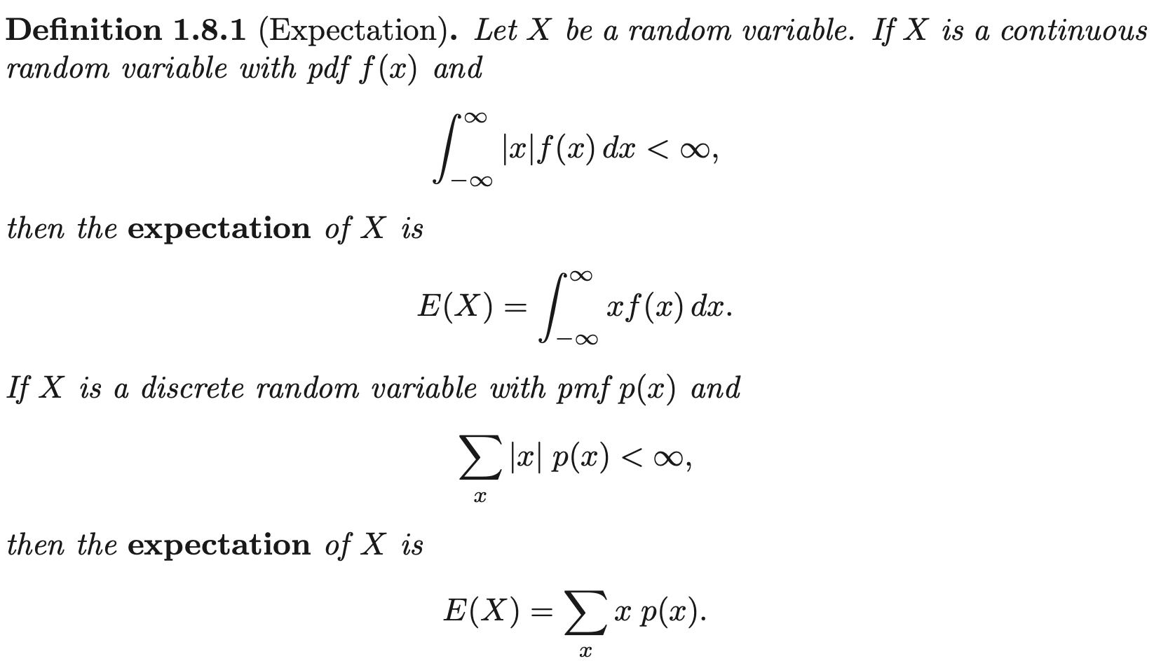
Sometimes, the expectation \(E[x]\) is called the mathmematical expectation of \(X\), the expected value of \(X\) or the mean of \(X\). When the name mean is used, we often denote the \(E[X]\) by \(\mu\).
Reference
- D. P. Bertsekas and J. N. Tsitsiklis, Introduction to Probability, NH, Nashua:Athena Scientific, 2008.