probability (2)
Probability Background (2)
Distribution of Two Random Variables
Intuitive Example:
Let our experiment be flipping a coin 3 times. Then our sample space \(\Omega = \{HHH, THH, TTH, TTT, THT, HTH, HTT, HHT\}\). Let \(X_1\) be the number of head on the first two tosses and \(X_2\) be the number of heads on all three tosses. Then, our interest can be represented by the pair of random variables \((X_1, X_2)\), for example \((X_1 (HTH), X_2(HTH)) = (1, 2)\). Continuing this way, \(X_1, X_2\) are real-valued functions defined on the sample space \(\Omega\), which take the outcome and map from sample space to ordered number pairs: \[\mathbb{D} = \{(0, 0), (0, 1), (1, 1), (1, 2), (2, 2), (2, 3)\}\]
One the other hand, we can regard this ordered pair of functions as a vector function \(f: \Omega \rightarrow \mathbb{D} \subset \mathbb{R}^2\) defined by \(f(x) = <X_1(x), \; X_2(x)>, \quad x \in \Omega\).
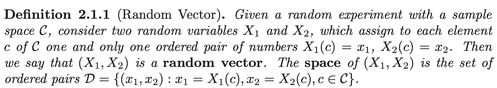
We often denote random vectors using vector notations \(\mathbf{X} = (X_1, X_2)^{\prime}\) as a column vector.
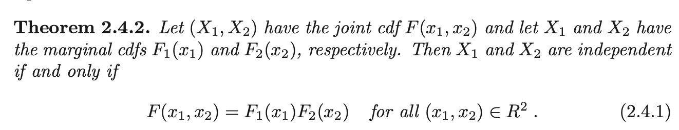
Let \(\mathbb{D}\) be the range space of \((X_1, X_2)\). Let \(A\) be a subset of \(\mathbb{D}\). We can uniquely define the distribution of this random vector \(P_{X_1, X_2}\) in terms of the CDF:
\[F_{X_1, X_2} (x_1, x_2) = P_{X_1, X_2}((X_1 \leq x_1) \cap (X_2 \leq x_2)) = P_{X_1, X_2}(X_1 \leq x_1, \; X_2 \leq x_2)\]
For all \((x_1, x_2) \in \mathbb{R}^2\). At the same time:
\[P_{X_1, X_2}(a_1 < X_1 \leq b_1, \; a_2 < X_2 \leq b_2) = F_{X_1, X_2} (b_1, b_2) - F_{X_1, X_2} (a_1, b_2) - F_{X_1, X_2} (b_1, a_2) + F_{X_1, X_2} (a_1, a_2)\]
Hence, all induced probabilities can be formulated in terms of the cdf. We often call this cdf the joint cumulative distribution.
Discrete Random Vector
A random vector \((X_1, X_2)\) is discrete random vector if its range space \(\mathbb{D}\) is finite or countable. Hence, \(X_1\) and \(X_2\) are both discrete. The joint probability mass function of \((X_1, X_2)\) \(p_{X_1, X_2}\) is defined by:
\[p_{X_1, X_2} (x_1, x_2) = P(\{c_1: X_1 (c_1) = x_1\} \cap \{c_2: X_2 (c_2) = x_2\}) = P(X_1 = x_1, X_2 = x_2)\]
for all \((x_1, x_2) \in \mathbb{D}\). The pmf uniquely defines the cdf, it also is characterized by the two properties:
\[0 \leq p_{X_1, X_2} (x_1, x_2) \leq 1, \quad \quad \underset{D}{\sum \sum} p_{X_1, X_2} (x_1, x_2) = 1\]
For an event \(B \subset \mathbb{D}\), we have:
\[P_{X_1, X_2} (B) = P((X_1, X_2) \in B) = \underset{B}{\sum \sum} p_{x_1, X_2} (x_1, x_2)\]
The support of a discrete random vector \((X_1, X_2)\) is defined as all points \((x_1, x_2)\) in the range space of \((X_1, X_2)\) such that \(p_{X_1, X_2} (x_1, x_2) > 0\).
Continuous Random Vector
We say a random vector \((X_1, X_2)\) with range space \(\mathbb{D}\) is of the continuous type if its cdf \(F_{X_1, X_2} (x_1, x_2)\) is continuous:
\[F_{X_1, X_2} (x_1, x_2) = \int^{x_1}_{-\infty} \int^{x_2}_{-\infty} f_{X_1, X_2} (w_1, w_2) dw_1 dw_2\]
For all \((x_1, x_2) \in \mathbb{R}^2\). We call \(f_{X_1, X_2}\) the joint probability density function of \((X_1, X_2)\). Then:
\[\frac{\partial^2 F_{X_1, X_2} (x_1, x_2)}{\partial x_1 \partial x_2} = f_{X_1, X_2} (x_1, x_2)\]
The pdf is essentially characterized by the two properties:
\[0 \leq f_{X_1, X_2} (x_1, x_2), \quad \quad \int^{\infty}_{-\infty} \int^{\infty}_{-\infty} f_{X_1, X_2} (x_1, x_2) dx_1dx_2= 1\]
Then, the probability distribution \(P_{X_1, X_2}\) is defined as:
\[P_{X_1, X_2} (A) = P((X_1, X_2) \in A) = \underset{A}{\int \int} f_{X_1, X_2} (x_1, x_2) dx_1dx_2\]
Note that \(P((X_1, X_2) \in A)\) is just the volumn under the surface (graph) \(z = f_{X_1, X_2} (x_1, x_2)\) over the set \(A\) (uncountable).
For continuous random vector the support of \((X_1, X_2)\) contains all points \((x_1, x_2)\) for which \(f(x_1, x_2) > 0\)
Marginal Distributions
Let \((X_1, X_2)\) be a random vector, we can obtain their individual distributions in terms of the joint distribution.
Consider events which defined the cdf of \(X_1\) at \(x_1\) is \(\{X_1 \leq x_1\}\), in scenario of random vector, this is the same as no limitation on \(X_2\):
\[\{X_1 \leq x_1\} \cap \{-\infty < X_2 < \infty\}\]
Taking the joint probability:
\[P(\{X_1 \leq x_1\} \cap \{-\infty < X_2 < \infty\}) = F_{X_1} (x_1) = \lim_{x_2 \rightarrow \infty} F_{X_1, X_2} (x_1, x_2)\]
For all \(x_1 \in \mathbb{R}\).
Marginal PMF
Now, we have the relationship between the cdfs. Let \(\mathbb{D}_1\) be the support of \(X_1\) and \(w_1 \in \mathbb{D}_1\), let \(\mathbb{D}_2\) be the support of \(X_2\) and \(x_2 \in \mathbb{D}_2\), we can extend pmf:
\[P(\{X_1 \leq x_1\} \cap \{-\infty < X_2 < \infty\}) = \sum_{w_1 \leq x_1} \sum_{x_2 \in \mathbb{D}_2} p_{X_1, X_2} (w_1, x_2)\]
Then, by the uniqueness of cdfs, the quantity \(\sum_{x_2 \in \mathbb{D}_2} p_{X_1, X_2} (w_1, x_2)\) is the pmf of \(X_1\) evaluated at \(w_1\):
\[p_{X_1}(x_1) = \sum_{x_2 \in \mathbb{D}_2} p_{X_1, X_2} (x_1, x_2)\]
For all \(x_1 \in \mathbb{D}_{1}\).
That is, to find \(p_{X_1}(x_1)\) we can fix \(x_1\) and sum \(p_{X_1, X_2}\) over all the values of \(x_2\). Same is for \(X_2\). These individual pmfs are called the marginal pmfs.
Marginal PDF
For continuous case:
\[P(\{X_1 \leq x_1\} \cap \{-\infty < X_2 < \infty\}) = \int^{x_1}_{-\infty} \int^{\infty}_{-\infty} f_{X_1, X_2} (w_1, x_2) dx_2 dw_1\]
Then, by the uniqueness of cdfs, the quantity in braces must be the pdf of \(X_1\), evaluated at \(w_1\):
\[f_{X_1} (x_1) = \int^{\infty}_{-\infty} f_{X_1, X_2} (x_1, x_2) dx_2\]
That is, in the continuous case the marginal pdf of \(X_1\) is found by integrating out \(x_2\). Same is for \(X_2\)
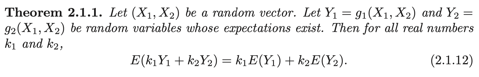
Expectation
Let \((X_1, X_2)\) be continuous random vector, let \(Y = g(X_1, X_2)\) where \(g: \mathbb{R}^2 \rightarrow \mathbb{R}\). Then the expectation of \(Y\), \(E[Y]\) exists if:
\[\int^{\infty}_{-\infty}\int^{\infty}_{-\infty} |g(x_1, x_2)| f_{X_1, X_2} (x_1, x_2) dx_1 dx_2 < \infty\]
Then,
\[E[Y] = \int^{\infty}_{-\infty}\int^{\infty}_{-\infty} g(x_1, x_2) f_{X_1, X_2} (x_1, x_2) dx_1 dx_2\]
Likewise, if \((X_1, X_2)\) is discrete, then:
\[E[Y] = \sum_{x_1} \sum_{x_2} g(x_1, x_2) p_{X_1, X_2} (x_1, x_2)\]
The expectation of function of individual random variable \(X_1\) can be found in two ways:
\[E[g(X_1)] = \int^{\infty}_{-\infty}\int^{\infty}_{-\infty} g(x_1) f_{X_1, X_2} (x_1, x_2) dx_1 dx_2 = \int^{\infty}_{-\infty} g(x_1) f_{X_1} (x_1) dx_1\]
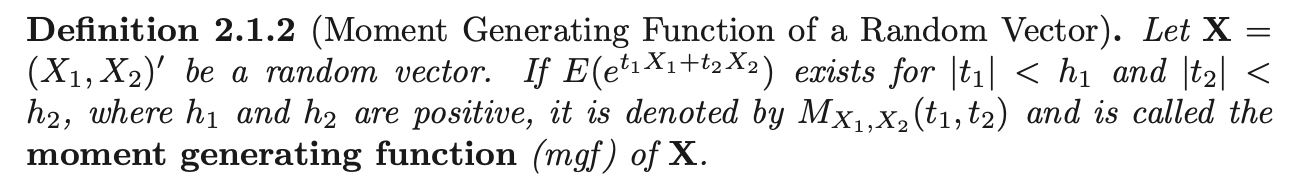
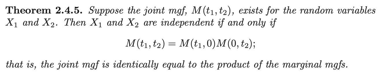
If moment generating function exists, then it uniquely determines the distribution of random vector \(\mathbf{X}\). Let \(\mathbf{t} = (t_1, t_2)^{\prime}\), then the moment generating function can be rewritten as:
\[M_{X_1, X_2} (\mathbf{t}) = E[e^{\mathbf{t^{\prime}} \mathbf{X}}]\]
With \(t_2 = 0\) or \(t_1 = 0\), we recover the MGFs for individual random variables.
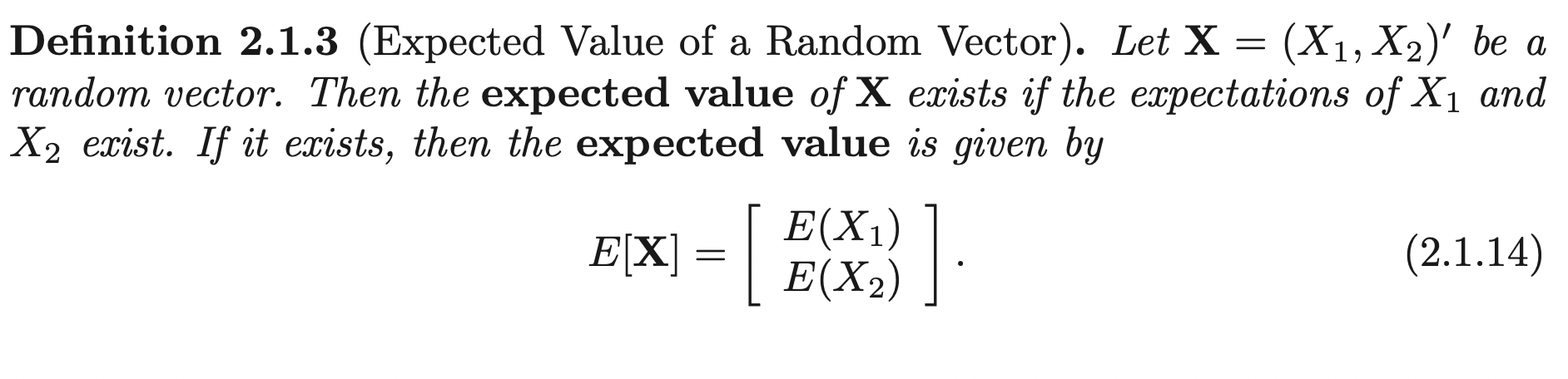
This is saying that, the expectation of a random vector is a vector function of expectation.
Transformation: Bivariate Random Variables
Let \(X_1, X_2\) denote random variables of the discrete type, which have the joint pmf \(p_{X_1, X_2} (x_1, x_2)\) that is positive on the support set \(S\). Let \(y_1 = u_1(x_1, x_2)\) and \(y_2 = u_2(x_1, x_2)\) define a one-to-one transformation that maps \(S\) onto \(T\). The joint pmf of the two new random variables \(Y_1 = u_1 (X_1, X_2)\) and \(Y_2 = u_2(X_1, X_2)\) is given by:
\[ p_{Y_1, Y_2}(y_1, y_2)= \begin{cases} p_{X_1, X_2} (w_1(y_1, y_2), w_2 (y_1, y_2)), \quad &(y_1, y_2) \in T\\ 0, \quad &o.w \end{cases} \]
Where \(w_1(y_1, y_2) = x_1\), \(w_2(y_1, y_2) = x_2\) is the single-valued inverse of \(y_1 = u_1(x_1, x_2)\) and \(y_2 = u_2 (x_1, x_2)\) (form function of \(x_1\) and \(x_2\) using \(y_1\) and \(y_2\)).
Conditional Distributions and Expectations
Discrete Conditional PMF
Let \(X_1\) and \(X_2\) denote random variables of the discrete type, which have the joint pmf defined to be \(p_{X_1, X_2} (x_1, x_2)\) that is positive on the support set \(S\) and is zero elsewhere. Let \(p_{X_1} (x_1)\) and \(p_{X_2} (x_2)\) denote, respectively the marginal probability mass function of \(X_1\) and \(X_2\). Let \(x_1\) be a point in the support of \(X_1\), then \(p_{X_1} (x_1) > 0\). We have:
\[P(X_2 = x_2 | X_1 = x_1) = \frac{P(X_1=x, X_2=x_2)}{P(X_1 = x_1)} = \frac{p_{X_1, X_2}(x_1, x_2)}{p_{X_1}(x_1)}\]
For all \(x_2\) in the support of \(S_{X_2}\). Then we define this function as:
\[p_{X_2 | X_1} (x_2 | x_1) = \frac{p_{X_1, X_2}(x_1, x_2)}{p_{X_1}(x_1)}, \quad x_2 \in S_{X_2}\]
For any fixed \(x_1\) with \(p_{X_1} (x_1) > 0\), this function has the conditions of being a pmf of the discrete type becuase:
\(p_{X_2 | X_1} (x_2 | x_1)\) is non-negative: \[p_{X_1} (x_1) > 0, \quad p_{X_1, X_2} (x_1, x_2) > 0, \; \forall (x_1, x_2) \in (S_{X_1} \times S_{X_2})\]
\(\sum_{x_2} p_{X_2 | X_1} (x_2 | x_1) = \sum_{x_2} \frac{p_{X_1, X_2}(x_1, x_2)}{p_{X_1}(x_1)} = \frac{\sum_{x_2}p_{X_1, X_2}(x_1, x_2)}{p_{X_1}(x_1)} = 1\)
We call \(p_{X_2 | X_1} (x_2 | x_1)\) the conditional pmf of discrete type of random variable \(X_2\) given the discrete type of random variable \(X_1 = x_1\). Similar formula can be derived for conditional pmf of \(X_1\) given \(X_2 = x_2\).
Continuous Conditional PMF
Now, let \(X_1\) and \(X_2\) be random variables of continuous type and have the joint pdf defined as \(f_{X_1, X_2} (x_1, x_2)\) and the marginal pdf defined as \(f_{X_1}(x_1)\) and \(f_{X_2} (x_2)\). When \(f_{X_1}(x_1) > 0\), we defined the function \(f_{X_1, X_2}\) as:
\[f_{X_2 | X_1} (x_2 | x_1) = \frac{f_{X_1, X_2}(x_1, x_2)}{f_{X_1}(x_1)}\]
Then, this function has the conditions of being a pdf of the continuous type becuase:
\(f_{X_2 | X_1} (x_2 | x_1)\) is non-negative: \[f_{X_1} (x_1) > 0, \quad f_{X_1, X_2} (x_1, x_2) > 0, \; \forall (x_1, x_2) \in (S_{X_1} \times S_{X_2})\]
\(\int^{\infty}_{-\infty} f_{X_2 | X_1} (x_2 | x_1) dx_2 = \int^{\infty}_{-\infty} \frac{p_{X_1, X_2}(x_1, x_2)}{p_{X_1}(x_1)} dx_2 = \frac{\int^{\infty}_{-\infty} f_{X_1, X_2}(x_1, x_2) dx_2}{f_{X_1}(x_1)} = 1\)
That is, this function is called conditional pdf of the continuous type of random variable \(X_2\), given that the continuous type of random variable \(X_1=x_1\). Similar formula can be derived for conditional pdf of \(X_1\) given \(X_2 = x_2\).
Since each of the pdfs \(f_{X_2 | X_1} (x_2 | x_1), f_{X_1 | X_2} (x_1 | x_2)\) is a pdf of one variable, each has all the propertiees of such a pdf. Thus we can compute probabilities and mathmetical expectations. If the random variables are of the continuous type, the probability:
\[P(a < X_2 < b | X_1 = x_1) = \int^{b}_{a} f_{X_2 | X_1} (x_2 | x_1) dx_2\]
This is called the conditional probability that \(a < X_2 < b\), given that \(X_1 = x_1\)
Conditional Expectation and Variance
If \(u(X_2)\) is a function of \(X_2\), the conditional expectation (continuous case) of \(u(X_2)\), given that \(X_1=x_1\), if it exists, is given by:
\[E_{X_2 | X_1}[u(X_2) | X_1=x_1] = \int^{\infty}_{-\infty} u(x_2) f_{X_2 | X_2} (x_2 | x_1) dx_2\]
Notice that, the conditional expectation \(E_{X_2 | X_1}[X_2 | X_1=x_1]\) is function of \(x_1\). If they do exist, then \(E_{X_2 | X_1}[X_2 | X_1=x_1]\) is the mean and:
\[Var(X_2 | x_1) = E_{X_2 | X_1}[(X_2 - E_{X_2 | X_1}[X_2 | X_1=x_1])^2 | X_1 = x_1]\]
is the conditional variance of the conditional distribution of \(X_2\), given \(X_1 = x_1\).
The similar rule holds for conditional variance:
\[Var(X_2 | x_1) = E_{X_2 | X_1}[X_2^2 | X_1=x_1]- (E_{X_2 | X_1}[X_2 | X_1=x_1])^2\]
Double Expectation
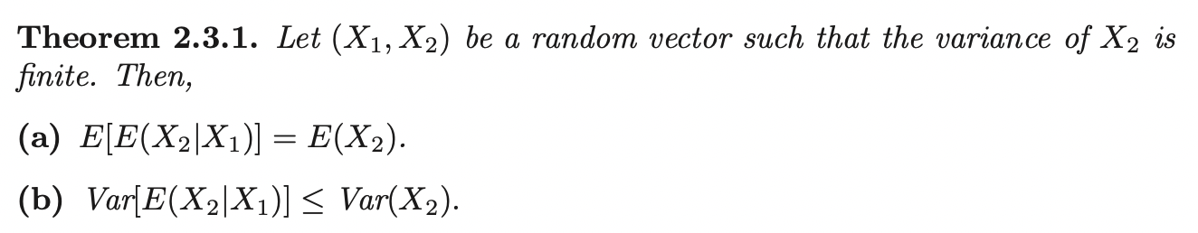
Proof:
\[\begin{aligned} E[X_2] &= \int^{\infty}_{-\infty} f_{X_2} (x_2) x_2 dx_2\\ &= \int^{\infty}_{-\infty} \int^{\infty}_{-\infty} x_2 f_{X_2, X_1} (x_2, x_1)dx_1 dx_2\\ &= \int^{\infty}_{-\infty} \int^{\infty}_{-\infty} x_2 f_{X_2, X_1} (x_2, x_1) dx_2 dx_1\\ &= \int^{\infty}_{-\infty}\int^{\infty}_{-\infty} x_2 f_{X_2 | X_1} (x_2 | x_1) f_{x_1} (x_1) dx_2 dx_1\\ &= \int^{\infty}_{-\infty} E_{X_2 | X_1}[X_2 | x_1] f_{x_1} (x_1) dx_2 dx_1\\ &= E_{X_1}[E_{X_2 | X_1}[X_2 | X_1]] \end{aligned}\]
Intuitively, this result could have this useful interpretation. Both the random variables \(X_2\) and \(E[X_2 | X_1]\) have the same mean \(\mu\). If we did not know \(\mu\), we can use either of the two random variables to guess. Since however, \(Var[X_2] \geq Var[E[X_2 | X_1]]\), we would put more reliance in \(E[X_2 | X_1]\) as a guess. That is, if we observe the pair \((x_1, x_2)\), we would prefer to use \(E[X_2 | x_1]\) over \(x_2\) to estimate \(\mu\).
Independent Random Variables
Let \(X_1\) and \(X_2\) denote the random variables of the continuous type that have the joint pdf \(f(x_1, x_2)\) and marginal probability density functions defined as \(f_1 (x_1)\) and \(f_2 (x_2)\) respectively. Suppose we have an instance where \(f_{X_2 | X_1} (x_2 | x_1)\) does not depend upon \(x_1\). Then the marginal pdf of \(X_2\) is
\[\begin{aligned} f_{X_2} (x_2) &= \int^{\infty}_{-\infty} f_{X_2, X_1} f(x_2, x_1) dx_1 \\ &= \int^{\infty}_{-\infty} f_{X_2 | X_1} f(x_2 | x_1) f_{X_1}(x_1) dx_1 \\ &= f_{X_2 | X_1} f(x_2 | x_1) \int^{\infty}_{-\infty} f_{X_1}(x_1) dx_1 \\ &= f_{X_2 | X_1} f(x_2 | x_1) \end{aligned}\]Then the joint pdf is:
\[f_{X_2, X_1} f(x_2, x_1) = f_{X_2 | X_1} f(x_2 | x_1) f_{X_1} (x_1) = f_{X_2} (x_2) f_{X_1} (x_1)\]
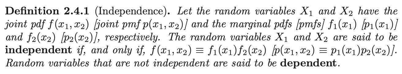
Theorem 2.4.1
Let random variables \(X_1\) and \(X_2\) have supports \(S_1\) and \(S_2\), respectively, and have the joint pdf \(f(x_1, x_2)\). Then \(X_1\) and \(X_2\) are independent if and only if \(f(x_1, x_2)\) can be written as a product of a nonnegative function of \(x_1\) and a nonnegative function of \(x_2\). That is: \[f(x_1, x_2) \equiv g(x_1) h(x_2)\]
Where \(g(x_1) > 0 \; \forall x_1 \in S_{1}\) and \(h(x_2) > 0, \; \forall x_2 \in S_{2}\), 0 elsewhere.
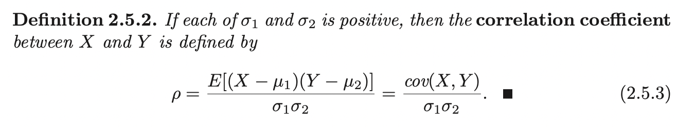
Correlation Coefficient
Let \((X, Y)\) denote a random vector. How do we know the correlation between them? There are many measures of dependence, we investigate a parameter \(\rho\) of the joint distribution of \((X, Y)\) which measures linearity between \(X\) and \(Y\).
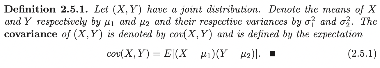
It follows by the linearity of expectation, that the covariance of \(X\) and \(Y\) can be expressed as:
\[Cov(X, Y) = E[XY - \mu_2 X - \mu_1 Y + \mu_1\mu_2] = E[XY] - \mu_1\mu_2\]


The converse is not true (i.e if \(Cov(X, Y) = 0 \implies X, Y\) are independent). However, the contrapositive is true:
If \(\rho \neq 0\), then \(X, Y\) are dependent.
Extension to Several Random Variables
We denote the random vector by n-dimensional column vector \(\mathbf{X}\) and the observed values (realization) of random vector by \(\mathbf{x}\). The joint cdf is defined to be:
\[F_{\mathbf{X}} (\mathbf{x}) = P[X_1 \leq x_1 ,....., X_n \leq x_n]\]
We say that the \(n\) random variables \(X_1\), ...., \(X_n\) are of the discrete type or of the continuous type and have a distribution of that type according to whether the joint cdf can be expressed as:
\[F_{\mathbf{X}} (\mathbf{x}) = \sum_{w_1 \leq x_1} .... \sum_{w_n \leq x_n} p_{\mathbf{X}}(w_1, ....., w_n)\]
or
\[F_{\mathbf{X}} (\mathbf{x}) = \int^{x_1}_{-\infty} .... \int^{x_n}_{-\infty} f(w_1, ....., w_n)dw_n .... dw_1\]
For continuous case:
\[\frac{\partial^n}{\partial x_1, ...., x_n} F_{\mathbf{X}} (\mathbf{x}) = f(\mathbf{x})\]
For the discrete case, the support set \(S\) of a random vector is all points in \(\mathbb{D}\) that have positive mass while for the continuous case these would be all points in \(\mathbb{D}\) that have positive mass that can be embedded in an open set of positive probability.
Expectation
Let \(\mathbf{X}\) be a \(n\) dimensional column random vector, let \(Y = u(\mathbf{X})\) for some function \(u\). As in the bivariate case, the expected value of a continuous random variable exists if the \(n\)-fold integral exists:
\[\int^{\infty}_{-\infty} .... \int^{\infty}_{-\infty} |u(\mathbf{x})|f(x_1, ....., x_n)dx_n .... dx_1\]
The expected value of a discrete random variable exists if the \(n\)-fold sum exists:
\[\sum_{x_1} .... \sum_{x_n} |u(\mathbf{x})|p_{\mathbf{X}}(x_1, ....., x_n)\]
Then the expectation is:
Discrete case: \[E[Y] = \sum_{x_1} .... \sum_{x_n} u(\mathbf{x})p_{\mathbf{X}}(x_1, ....., x_n)\]
Continuous case: \[E[Y] = \int^{\infty}_{-\infty} .... \int^{\infty}_{-\infty} u(\mathbf{x})f(x_1, ....., x_n)dx_n .... dx_1\]
Marginal Distribution
By an argument similar to the two-variable case, we have:
\[f_{X_1} (x_1) = \int^{\infty}_{-\infty} .... \int^{\infty}_{-\infty} f(x_1, ....., x_n)dx_n .... dx_2\]
\[p_{X_1} (x_1) = \sum_{x_2} .... \sum_{x_n} p_{\mathbf{X}}(x_1, ....., x_n)\]
Now, if we take subset of \(k\) where \(k < n\) from \(\mathbf{X}\), then we can define the Marginal pdf of subset of k variables.
Conditional Distribution
Similarly, we can extend the definition of a conditional distribution from bivariate conditional distribution.
Suppose, \(f_{X_1} (x_1) > 0\). Then we define the symbol \(f_{X_2,....,X_n | X_1} (x_2,.....,x_n | x_1)\) by the relation:
\[f_{X_2,....,X_n | X_1} (x_2,.....,x_n | x_1) = \frac{f_{\mathbf{X}} (\mathbf{x})}{f_{X_1} (x_1)}\]
Then \(f_{X_2,....,X_n | X_1} (x_2,.....,x_n | x_1)\) is called the joint conditional pdf of \(X_2, ...., X_n\) given \(X_1 = x_1\).
More general, the joint conditional pdf of \(n - k\) of the random variables, for given values of the remaining \(k\) variables, is defined as the joint pdf of the \(n\) variables divided by the marginal pdf of the particular subset group of \(k\) variables, provided that the latter pdf is positive.
Conditional Expectation
The conditional expectation of \(u(X_2, ...., X_n)\) given \(X_1 = x_1\) (continuous) is given by:
\[E[u(X_2, ...., X_n) | x_1] = \int^{\infty}_{-\infty} .... \int^{\infty}_{-\infty} u(x_2, ...., x_n) f_{X_2, ..., X_n | X_1}(x_2, ....., x_n | x_1)dx_n .... dx_2\]
Mutually Independent
The random variables \(X_1, ...., X_n\) are said to be mutually independent IFF
\[f_{\mathbf{X}}(\mathbf{x}) = f_{X_1} (x_1) .... f_{X_n} (x_n)\]
for the continuous case. Similar for discrete case.
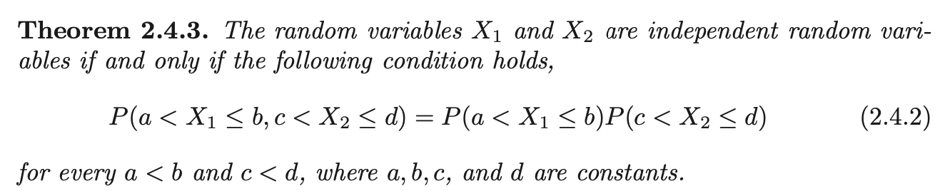
Suppose \(X_1, ...., X_n\) are mutually independent. Then,
CDF: \[P(a_1 < X_1 < b_1, a_2 < X_2 < b_2, ....., a_n < X_n < b_n) = P(a_1 < X_1 < b_1) .... P(a_n < X_n < b_n) = \prod^{n}_{i=1} P(a_i < X_i < b_i)\]
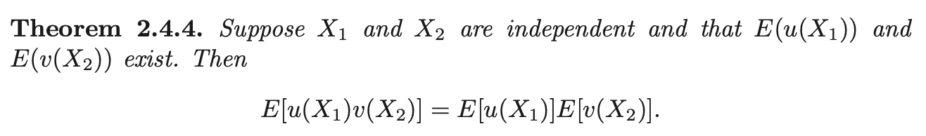
Expectation: \[E[u_1(X_1) ... u_n(X_n)] = E[u_1(X_1)] ... E[u_n (X_n)]\]
Pairwise Independent
If \(X_i, X_j, i \neq j\) are independent, we say that they are pairwise independent. If random variables are mutually independent, they are pairwise independent. However, the converse is false, pairwise independence does not imply mutual independence:
In addition, if several random variables are mutually independent and have the same distribution, we say that they are independent and identically distributed (i.i.d).