Dueling Network Architectures for DRL
Dueling Network Architectures for Deep Reinforcement Learning
Introduction
The authors introduce an innovating neural network architecture that is better suited for model-free RL. This paper advances a new network but uses already published algorithms.
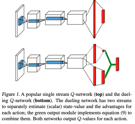
The proposed architecture is called dueling architecture, explicitly separates the representation of state values and state-dependent action advantages. The architecture consists of two streams that represent the value and advantage functions, while sharing a common convolutional feature learning module. The two streams are combined via a special aggregating layer to produce an estimate of the state-action value function \(Q\). This dueling network should be understood as a single Q network with two streams that replaces the popular single-stream Q-network in existing algorithms such as DQN. The dueling network automatically produces separate estimates of the state value function and advantage function, without any extra supervision.
Intuitively, the dueling architecture can learn which states are (or are not) valuable, without having to learn the effect of each action for each state. (by taking the gradient wrt to the input) It can more quickly identify the correct action during policy evaluation as redundant or similar actions are added to the learning problem.
Background
random variables have subscript \(t\), \(E[ g(x_t, a_t) | x_t=x, a_t] = f(x, a)\) is shorthanded as \(f(x, a) = E[g(x, a)]\)
In Atari domain, the agent perceives a video \(s_t\) consisting of M image frames \(s_t = (x_{t-M+1}, ..., x_t) \in S\) at time step \(t\). Then agent chooses an action from a discrete set \(a_t \in A\) and observes a reward signal \(r_t\) produced by the game emulator.
The agent seeks to maximize the expected discounted return where we define the discounted return as \(R_t = \sum_{\tau=t}^{\infty} \gamma^{\tau - t} r_{\tau}\) with \(\gamma \in [0, 1]\).
For an agent behaving to a stochastic policy \(\pi\), the values of the state-action pair \((s, a)\) and the state \(s\) are defined as:
\[Q^{\pi} (s, a) = E[R_t | s_t=s, a_t=a, \pi]\]
\[V^{\pi} (s) = E_{a_t \sim \pi(\cdot | s)}[R_t | s_t=s, \pi] = E_{a_t \sim \pi(\cdot | s)}[E[R_t | s_t, a_t, \pi] | s_t=s] = E_{a_t \sim \pi(\cdot | s)}[ Q^{\pi}(s, a_t)]\]
We know that we can rewrite \(Q^{\pi}\) as:
\[Q^{\pi} (s, a) = E_s^{\prime} [r + \gamma E_{a^{\prime}}[Q(s^{\prime}, a^{s^{\prime}}) | s^{\prime}] | s, a, \pi]\]
We also define:
\[Q^{*} (s, a) = max_{\pi} Q^{\pi} (s, a), \forall (s, a) \in S X A\]
Then:
\[V^{*} (s) = max_{a} Q^{*} (s, a)\]
And,
\[Q^{*}(s, a) = E_{s^{\prime}} [r + \gamma max_{a^{\prime}} Q^{*} (s^{\prime}, a^{\prime}) | s, a]\]
The advantage function is denoted as:
\[A^{\pi} (s, a) = Q^{\pi} (s, a) - V^{\pi} (s)\]
\[E_{a}[A^{\pi} (s, a) | s] = E_{a}[Q^{\pi} (s, a) | s] - V^{\pi} (s) = 0\]
This means that the advantage at state \(s\) weighted by policy \(\pi\) is 0. Intuitively, the advantage function measures the relative importance for each action.
Dueling Network Architecture
Instead of following the convolutional layers with a single sequence of fully connected layers, they instead use two sequences (streams) of fully connected layers. The streams are constructed such that they have the capability of providing separate estimates of the value and advantage functions. Finally , the two streams are combined to produce a single output \(Q\) function.
From the advantage expression, we know that
\[Q^{\pi} (s, a) = V^{\pi} (s) + A^{\pi} (s, a)\]
If the policy is the deterministic policy, \(a^{*} = argmax_{a^{\prime} \in A} Q(s, a^{\prime})\), then:
\[E_{a}[Q^{\pi} (s, a)] = Q^{\pi} (s, a^{*}) = V^{\pi} (s)\] and hence \[A^{\pi}(s, a^{*}) = 0\]
Let \(V(s; \theta, \beta), A(s, a; \theta, \alpha), Q(s, a; \theta, \alpha, \beta)\) be parametrized version of \(V, A, Q\) respectively. \(\theta\) are the shared parameters, \(\alpha\) and \(\beta\) are the stream parameters for \(V, A\). We can calculate \(Q\) directly using the formula:
\[Q(s, a; \theta, \alpha, \beta) = V(s; \theta, \beta) + A(s, a; \theta, \alpha)\]
However, these functions are just estimates of the true values, therefore are unidentifiable in the sense that given \(Q\) we can not recover \(V, A\) uniquely. (ie. given \(Q(s, a)\) what is \(V(s), A(s, a)\)?)
To solve the problem, we can force the advantage function to have zero advantage at some chosen action, in this case the greedy action:
\[Q(s, a; \theta, \alpha, \beta) = V(s; \theta, \beta) + A(s, a; \theta, \alpha) - max_{a^{\prime}} A(s, a^{\prime}; \theta, \alpha)\]
Thus, if \(a^{*} = argmax_{a^{\prime} \in A} Q(s, a^{\prime})\), then
\[Q(s, a^{*}; \theta, \alpha, \beta) = V(s; \theta, \beta)\]
We can determine the \(V\) given \(Q\).
Or, we can have:
\[Q(s, a; \theta, \alpha, \beta) = V(s; \theta, \beta) + A(s, a; \theta, \alpha) - \frac{1}{|A|} \sum_{a^{\prime}} A(s, a^{\prime}; \theta, \alpha)\]
Take the expectation or average of \(Q\):
\[E[Q(s, a; \theta, \alpha, \beta)] = V(s; \theta, \theta)\]
On the one hand this loses the original semantics of \(V\) and \(A\) because they are now off-target by a constant, but on the other hand it increases the stability of the optimization. Note that while subtracting the mean or max helps with the identifiability, it does not change the relative rank of \(A, Q\), so the greedy action.
Discussion
The advantage of the dueling architecture lies partly in its ability to learn the state-value function efficiently. With every update of the \(Q\) values in the dueling architecture, the value stream \(V\) is updated – this contrasts with the updates in a single-stream architecture where only the value of one of actions is updated, the values of other actions are untouched. The advantage of the dueling architecture over single-stream \(Q\) networks grows when the number of actions is large.
Implementation
One implementation of Dueling Architecture in PARL using PaddlPaddle for Atari Games
1 |
|