Calculus (1)
Multivariate Calculus (1)
Fundamental Theorem of Calculus
If \(f\) is continuous and \(F\) is indefinite integral of \(f\) (i.e \(F^{\prime} = f\) or \(\int f(x) dx = F(x) + c\), without bounds) on closed interval \([a, b]\), then:
- \(\int^{b}_{a} f(x) dx = F(b) - F(a)\)
- \(\frac{d}{dx}\int^{x}_{a} f(t)dt = F^{\prime}(x) - F^{\prime}(a) = F^{\prime} (x) = f(x)\)
Definition of Integral
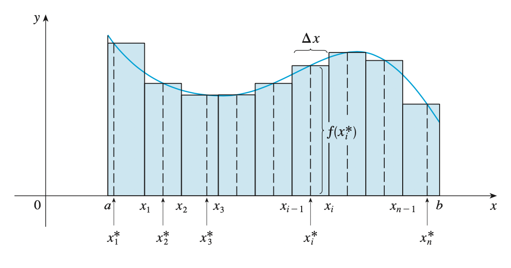
If \(f(x)\) is defined for \(a \leq x \leq b\), we start by dividing the interval \([a, b]\) into \(n\) sub-intervals \([x_{i - 1}, x_{i}]\) of equal width \(\Delta x = \frac{b - a}{n}\) and we choose sample points \(x^{*}_i\) in these subintervals. Then we form the Riemann sum:
\[\sum^{n}_{i=1} f(x^{*}_n) \Delta x\]
Then by taking the limit \(n \rightarrow \infty\), we have the definite integral of \(f\) from \(a\) to \(b\):
\[\int^{b}_{a} f(x) dx = \lim_{n \rightarrow \infty} \sum^{n}_{i=1} f(x^{*}_n) \Delta x\]
In the special case where \(f(x) \leq 0\), we can interpret the Riemann sum as the sum of the areas of the approximating rectangles, and \(\int^{b}_{a} f(x) dx\) represents the area under the curve \(y = f(x)\) from \(a\) to \(b\).
Vectors and the Geometric of Space
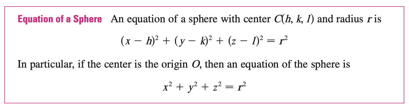
Equation of a sphere
By definition, a sphere is the set of all points \(P(x, y, z)\) whose distance from \(C\) is \(r\), where \(C\) is the center \(C(h, k, l)\). Thus, \(P\) is on the sphere if and only if
\[|PC| = r \implies |PC|^2 = r^2\]
\[(x - h)^2 + (y - k)^2 + (z - l)^2 = r^2\]
Vectors
The term vector is used by scientists to indicate a quantity that has both magnitude and direction.
In three dimensions, the vector \(a = \vec{OP}\) is the position vector of the point \(P\). We can think of all geometric vectors as representation of the position vector of the point \(P\).
Dot product
Proof
Recall the law of cosines for vector \(a\) and \(b\) and their difference \(a - b\):
\[|a - b|^2 = |a|^2 + |b|^2 - 2|a||b|\cos\theta\]
If we expand left side:
\[|a - b|^2 = (a - b) \cdot (a - b) = |a|^2 + |b|^2 - 2 a \cdot b\]
Then we have:
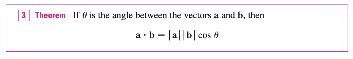
\[|a|^2 + |b|^2 - 2 a \cdot b = |a|^2 + |b|^2 - 2|a||b|\cos\theta \implies a \cdot b = |a||b|\cos \theta\]
If two vectors are perpendicular or orthogonal \(\Longleftrightarrow\) the angle between them is \(\theta = 90^\circ\) and \(a \cdot b = 0\)
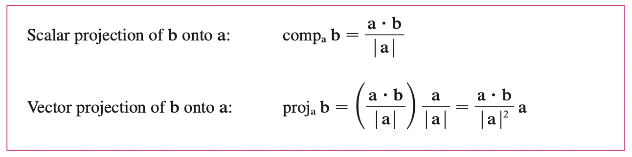
Projections
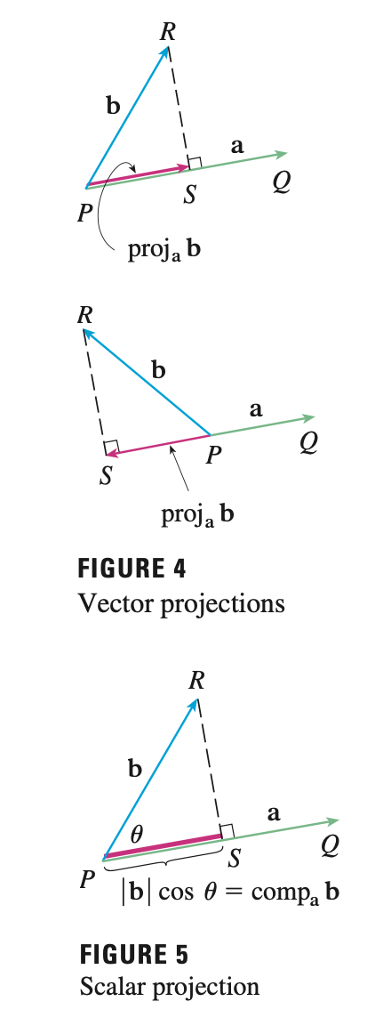
The vector projection of \(b\) onto \(a\) is denoted as \(proj_a b\). The \(comp_a b\) is defined to be the signed magnitude of the vector projection.
\(\cos \theta = \frac{adjacent}{hypotenuse} \implies\) the magnitude of the project vector is \(comp_{a} b = |b| \cos \theta\).
Recall that the dot product:
\[a \cdot b = |a|(|b|\cos \theta)\]
So:
\[com_{a} b = \frac{a \cdot b }{|a|}\]
Remember that \(proj_a b\) is a vector, we need to add direction of \(a\) which is \(\frac{a}{|a|}\) to the magnitude \(comp_a b\):
\[proj_a b = \frac{a \cdot b }{|a|} \frac{a}{|a|} = \frac{a \cdot b}{|a|^2} a\]
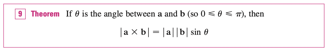
Cross Product
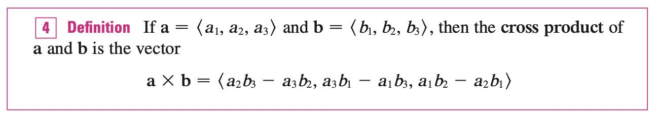
The cross product of \(a\) and \(b\) is a vector. Note that \(a \times b\) is only defined when \(a\) and \(b\) are three-dimensional vectors.

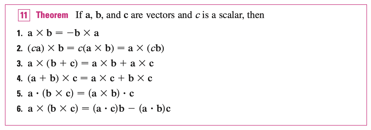
Two non-zero vectors \(a, b\) are parallel if and only if \(a \times b = 0\)
Equations of Lines and Planes
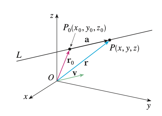
A line on xy-plane is determined when a point on the line and the direction of the line. Likewise, a line \(L\) in 3 dimensional space is determined when we know a point \(P_0 (x_0, y_0, z_0)\) on \(L\) and the direction of \(L\).
In 3 d space the direction of the line is described as a vector, so we let \(v = \vec{OV}\) be a vector parallel to \(L\). Let \(P(x, y, z)\) be an arbitrary point on \(L\) and let \(r_0 = \vec{OP_0}\) and \(r= \vec{OP}\) be the position vectors of Let \(a = \vec{P_0P}\), then
\[\vec{P_0P} = \vec{OP} - \vec{OP_0} \implies r = r_0 + a\]
Since \(a, v\) are parallel vectors, there is a scalar such that \(a = tv\). Thus:
\[r = r_0 + tv\]
This is the vector equation of \(L\) in 3 d. Each value of the parameter \(t\) gives the position vector \(r\) of a point on \(L\). So the line in 3 d is represented by a position vector on the line and a scalar multiple of direction vector \(tv\).
In component form \(r = <x, y, z>, r_0 = <x_0, y_0, z_0>, v=<a, b, c>\), each component is called parametric equation of the line \(L\) through point \(P_0\):
\[<x, y, z> = <x_0 + ta, y_0 + tb, z_0 + tc>\]
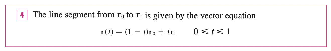
In general, we know that the vector equation of a line through the tip of the vector \(r_0\) in the direction of a vector \(v\) is \(r(t) = r_0 + tv\). If the line also passes through the tip of \(r_1\), then we can take \(v = r_1 - r_0\) because \(v = r_1 - r_0\) is parallel to the line \(L\), thus satisfies the vector equation of line:
\[r(t) = r_0 + tv = r_0 + t(r_1 - r_0)\]
If \(t = 1 \implies r = r_1\), if \(t = 0 \implies r = r_0\), the line segment from $r_0 $ to \(r_1\) is ten given by the parameter interval \(0 \leq t \leq 1\):
Planes
Although a line in space is determined by a point and a direction, a plane in space is more difficult to describe.
A plane in the space is determined by a point \(P_0\) in the plane and a vector \(n\) that is orthogonal to the plane. This orthogonal vector \(n\) is called a normal vector.
Let \(P(x, y, z), P_0 (x_0, y_0, z_0)\) be an arbitrary point in the plane, and let \(r_0\) and \(r\) be the position vectors of \(P_0\) and \(P\). Then the vector \(r - r_0 = \vec{P_0 P}\) is on the plane. The normal vector \(n = <a, b, c>\) is orthogonal to every vector on the plane, that is:
\[n \cdot (r - r_0) = 0\]
We can rewrite this as:
\[n \cdot r = n \cdot r_0\]
Either of these equations are called a vector equation of the plane.
The scalar equation of the plane through \(P_0\) with normal vector \(n\) can be written as:
\[<a, b, c> \cdot <x - x_0, y - y_0, z - z_0> = 0 \implies a (x - x_0) + b (y - y_0) + c (z - z_0) = 0\]
By collecting terms, we can have:
\[ax + by + cz + d = 0\]
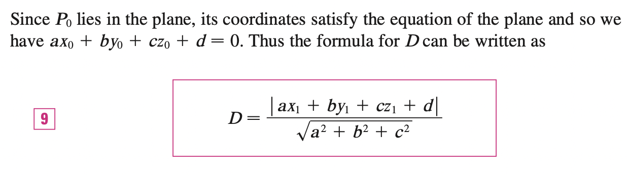
Where \(d = -(ax_0 + by_0 + cz_0)\). If \(a, b, c\) are not all zero, this equation can represent the plane.
Two planes are parallel if their normal vectors are parallel. If two planes are not parallel, then they intersact in a straight line and the angle between them is defined as the acute angle between their normal vectors.
The distance to plane
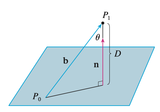
We know that the \(D = comp_n b = \frac{n \cdot b}{|n|}\), since the distance is positive, we need to find \(|comp_n b|\):
\[|D| = |comp_n b| = \frac{|n \cdot b|}{|n|}\]
Vector Functions
Vector Functions and Space Curves
In general, a function is a rule that assigns to each element in the domain an element in the range. A vector-valued function, is simply a function whose domain is a set of real numbers and whose range is a set of vectors.
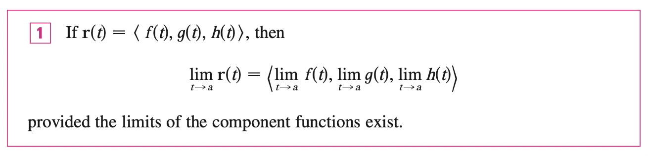
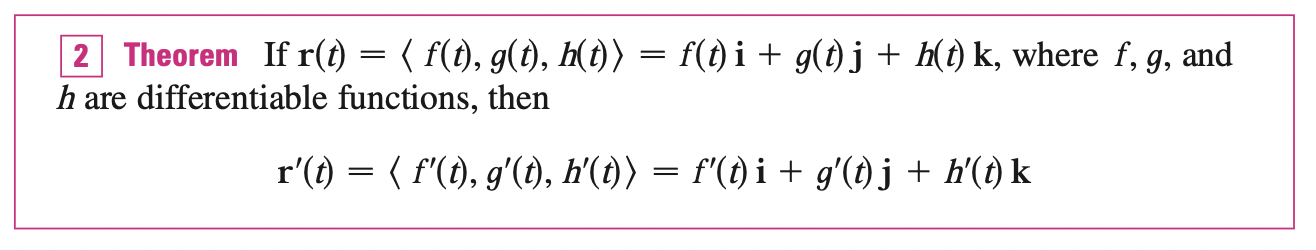
We are most interested in vector functions \(r\) whose values are three-dimensional vectors. This means that for every number \(t\) in the domain of \(r\) three is a unique vector in \(V_3\) denoted by \(r(t)\). If \(f(t), g(t), h(t)\) are the components of the vector \(r(t)\), then \(f, g\) and \(h\) are real-valued functions called the component functions of \(r\) and we can write:
\[r(t) = <f(t), \;g(t), \;h(t)>\]
if \(\lim_{t \rightarrow \infty} r(t) = L\), then this is equivalent to saying that the length and direction of the vector \(r(t)\) approach the length and direction of the vector \(L\).
A vector function \(r\) is continuous at \(a\) if:
\[\lim_{t \rightarrow a} r(t) = r(a)\]
That is, \(r(t)\) is continuous at \(a\) if and only if all the components are continuous at \(a\).
Derivatives and Integrals of Vector Functions
Derivatives
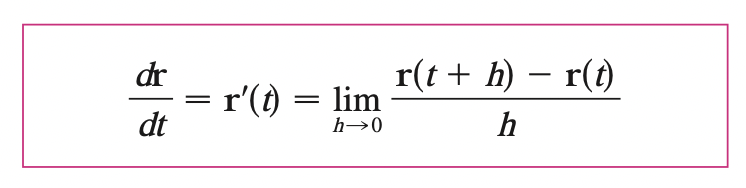
If the limit exists, let \(P, Q\) with position vector \(r(t), r(t + h)\), then \(r(t + h) - r(t)\) is the vector between them, \(\frac{r(t + h) - r(t)}{h}\) has same direction as \(r(t + h) - r(t)\). As \(h \rightarrow 0\), \(r(t + h)\) gets closer to \(r(t)\) so \(\frac{r(t + h) - r(t)}{h}\) becomes the tangent vector to the curve defined by \(r\) at the point \(P\).
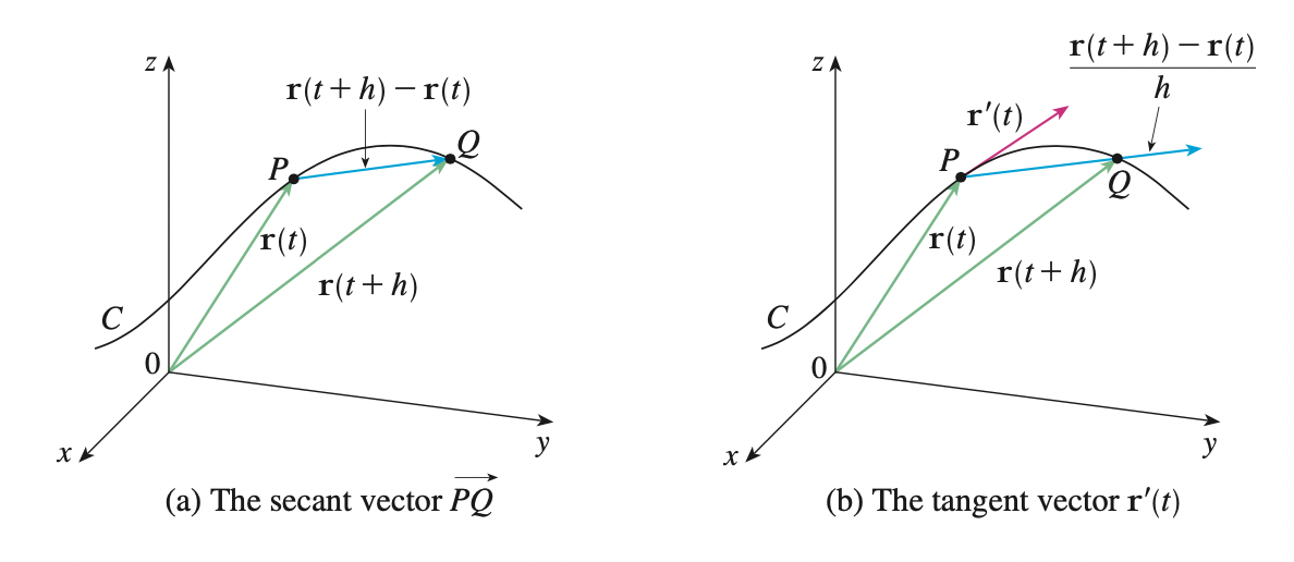
The tangent line at \(P\) is defined to be the line through \(P\) parallel to the tangent vector \(r^{\prime}(t)\)
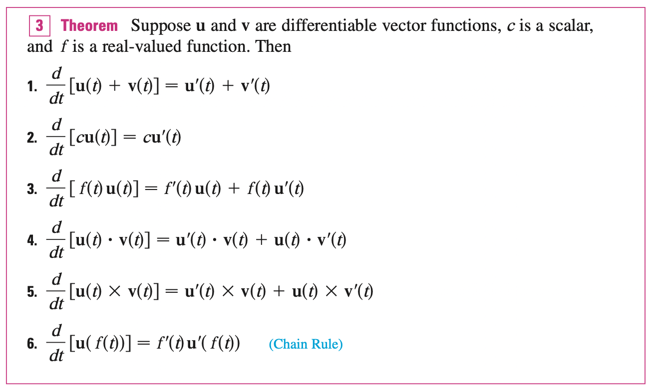
Differentiation Rules
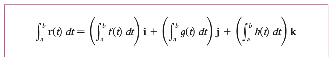
Integrals
Arc Length and Curvature
Suppose that the curve has the vector equation \(r(t) = <f(t), g(t), h(t)>, \; a\geq t \leq b\). The length of the space curve as t traverses exactly once from \(a\) to \(b\) can be shown:
\[L = \int^{b}_{a} \sqrt{[f^{\prime}(t)]^2 + [g^{\prime}(t)]^2 + [h^{\prime}(t)]^2} dt = \int^{b}_{a} |r^{\prime}(t)| dt\]
Where \(|r^\prime(t)| = \sqrt{[f^{\prime}(t)]^2 + [g^{\prime}(t)]^2 + [h^{\prime}(t)]^2}\) is the length of tangent vector at any point defined by space curve \(r(t)\).
Reparameterize a curve with respect to arc length
Let \(s(t)\) be the arc length between point \(r(a), r(t)\):
\[s(t) = \int^{t}_{a} |r^{\prime}(u)| du\]
Then by the fundamental theorem of calculus, we have:
\[s^{\prime}(t) = |r^{\prime}(t)|\]
By calculating \(|r^{\prime} (t)|\), and \(s(t)\) with \(t\) as function of \(s\), we can reparameterize the space curve by \(r(t(s))\).
Curvature
A parameterization \(r(t)\) is called smooth on an interval \(I\) if \(r^{\prime}\) is continuous and \(r^{\prime} (t) \neq 0\) on \(I\).
A curve is called smooth if it has a smooth parametrization. A smooth curve has no sharp corners or cusps when the tangent vector turns, it does so continuously.
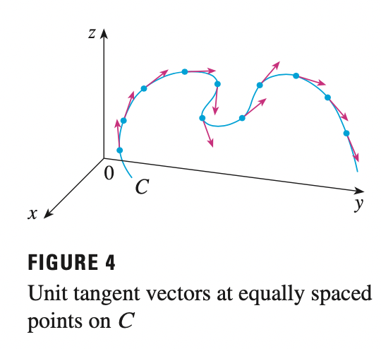
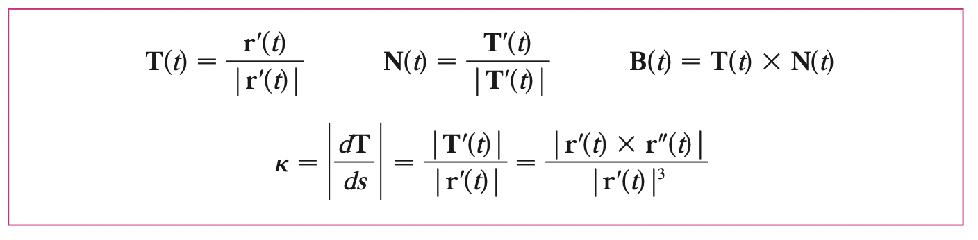
If \(C\) is a smooth curve defined by the vector function \(r\), the unit tangent vector \(T(t)\) is given by:
\[T(t) = \frac{r^{\prime} (t)}{|r(t)|}\]
and this indicates the direction of the curve.
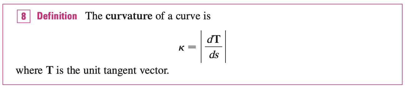
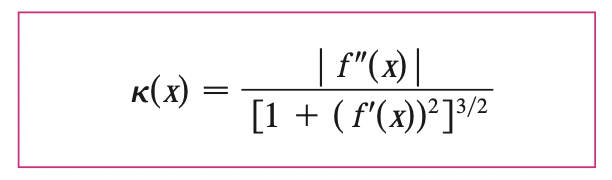
The curvature of \(C\) at a given point is a measure of how quickly the curve changes direction at that point. Specifically, we define it to be the magnitude of the rate of change of the unit tangent vector with respect to arc length.
\[\frac{dT}{dt} = \frac{dT}{ds} \frac{ds}{dt} \implies |\frac{dT}{ds}| = |\frac{\frac{dT}{dt}}{\frac{ds}{dt}}|\]
Remember \(\frac{ds}{dt} = |r^{\prime} (t)|\):
\[|\frac{dT}{ds}| = \frac{|T^{\prime} (t)|}{|r^{\prime} (t)|}\]
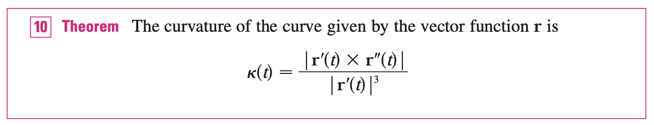
In general, the below formula is more convenient to apply:
In 2d case:
The Normal and Binormal Vectors
Since \(|T(t)| = 1 \implies T(t) \cdot T(t) = 1\), we have:
\[\frac{T(t) \cdot T(t)}{t} = T^{\prime}(t) \cdot T(t) + T^{\prime}(t) \cdot T(t) = 2 T^{\prime}(t) \cdot T(t) = 0\]
Thus, \(T^{\prime} (t) \cdot T(t) = 0\). \(T^{\prime} (t)\) is orthogonal to \(T(t)\). Note that \(T^{\prime} (t)\) is itself not a unit vector. But at any point where \(k \neq 0\) we can define the principal unit normal vector N(t) as:
\[N(t) = \frac{T^{\prime} (t)}{|T(t)|}\]
The vector \(B(t) = T(t) \times N(t)\) is called the binormal vector. It is perpendicular to both \(T\) and \(N\) and is also a unit vector at particular point.
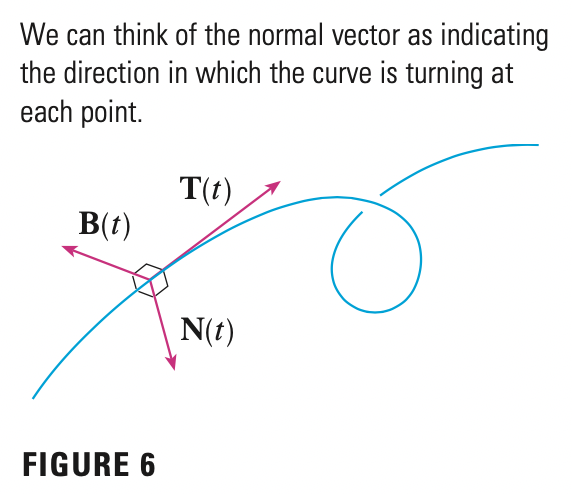
The plane determined by the normal and binormal vectors \(N\) and \(B\) at a point \(P\) on a curve \(C\) is called the normal plane of \(C\) at \(P\). It consists of all lines that are orthogonal to the tangent vector \(T\).
The plane determined by the vectors \(T\) and \(N\) is called the osculating plane of \(C\) at \(P\). It is the plane that comes closest to containing the part of the curve near \(P\).
Partial Derivatives
Functions of Several Variables
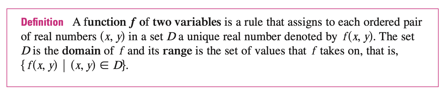
A function of two variables is just a function whose domain is a subset of \(\mathbb{R}^2\) and whose range is subset of \(\mathbb{R}\)
A function of three variables, \(f\), is a rule that assigns to each ordered triple \((x, y, z)\) in a domain \(D \in \mathbb{R}^3\) a unique real number denoted by \(f(x, y, z)\).
In general, function of any number of variables can be considered. A function of n variables is a rule that assigns a number \(z = f(x_1, ...., x_n)\) to an \(n\)-tuple \((x_1, x_2, ..., x_n)\) of real numbers. We denote by \(\mathbb{R}^{n}\) the set of all such \(n\)-tuples. Sometimes we will use vector notation to write such functions more compactly as \(f(\mathbf{x}), \quad \mathbf{x} = <x_1, ....., x_n>\).
In this view of the one to one correspondence between points \((x_1, ......, x_n)\) in \(\mathbb{R}^n\) and their position vectors \(\mathbf{x} = <x_1, ....., x_n>\). In general, we have three ways of looking at a function \(f\) defined on a subset of \(\mathbb{R}^n\):
- As a function of \(n\) real variables \(x_1, ....., x_n\)
- As a function of a single point variable \((x_1, ....., x_n)\)
- As a single vector variable \(\mathbf{x} = <x_1, ....., x_n>\)
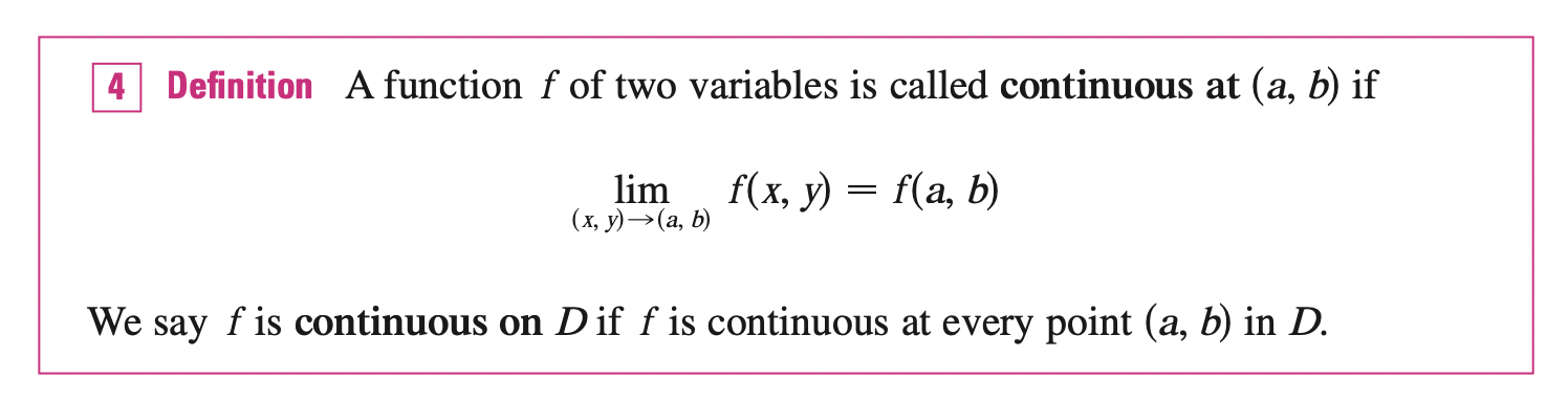
Limits and Continuity
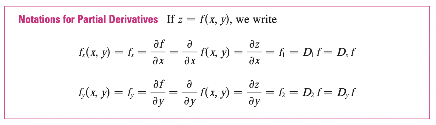
Partial Derivatives
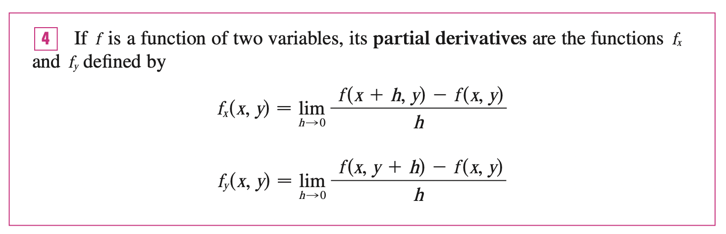
In general if \(f\) is a function of two variables \(x\) and \(y\), suppose we let only \(x\) vary while keeping \(y=b\) fixed. Then, we are really considering a function of a single variable \(x\), namely, \(g(x) = f(x, b)\). If \(g\) has a derivative at \(a\), then we call it the partial derivative of \(f\) with respect to \(x\) at \((a, b)\) and denote it by \(f_x (a, b)\). Thus,
Geometry View of Partial Derivatives
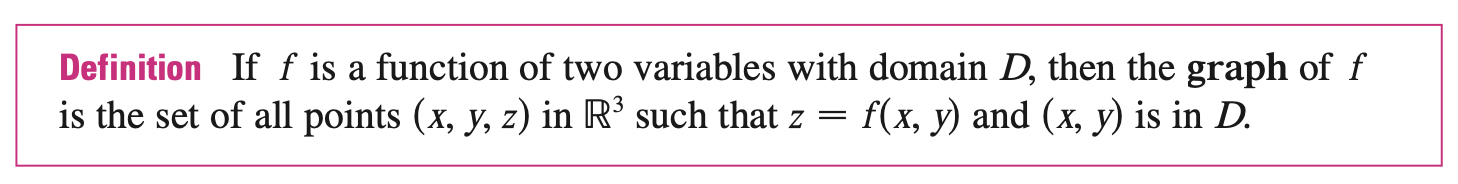
We recall that the equation \(z = f(x, y)\) represents a surface \(S\) (the graph of \(f\)) that maps points on \((x, y, 0)\) to \((x, y, z)\). By fixing \(y=b\), we have a curve \(C_1\) that is the vertical plane \(y=b\) intersecting \(S\). Likewise, the vertical plane \(x=a\) intersects \(S\) in a curve \(C_2\), both of curves \(C_1\), \(C_2\) passes through the point \((a, b, z)\).
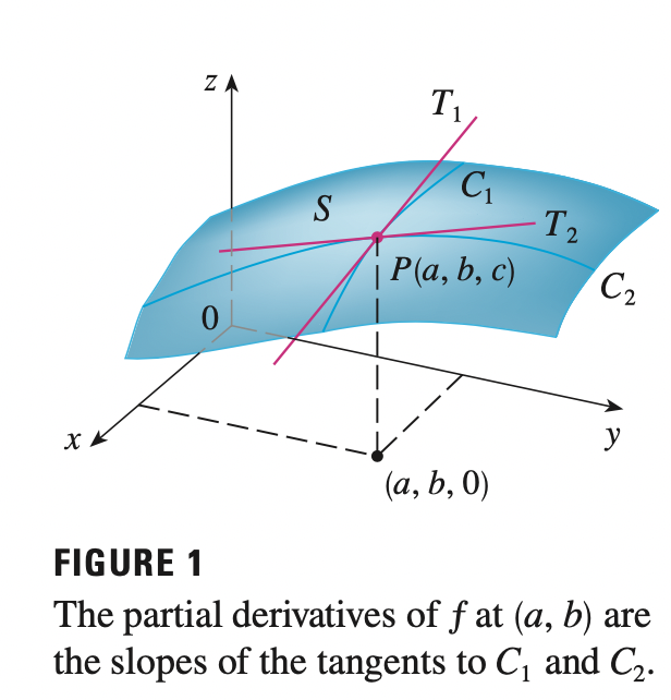
Thus, the partial derivatives \(f_x (a, b)\) and \(f_y(a, b)\) can be interpreted geometrically as the slopes of the tangent lines at \(P(a, b, z)\) to the curves \(C_1\), \(C_2\) of \(S\) in the planes \(y=b\) and \(x=a\)
The partial derivatives can also be interpreted as rate of changes. If \(z = f(x, y)\), then \(f_x\) represents the rate of change of \(f\) or \(z\) (\(z = f(x, y)\), to emphasize this is a function depends on \(x, y\)) with respect to \(x\) when \(y\) is fixed.
Tangent Planes and Linear Approximations
Tangent Planes
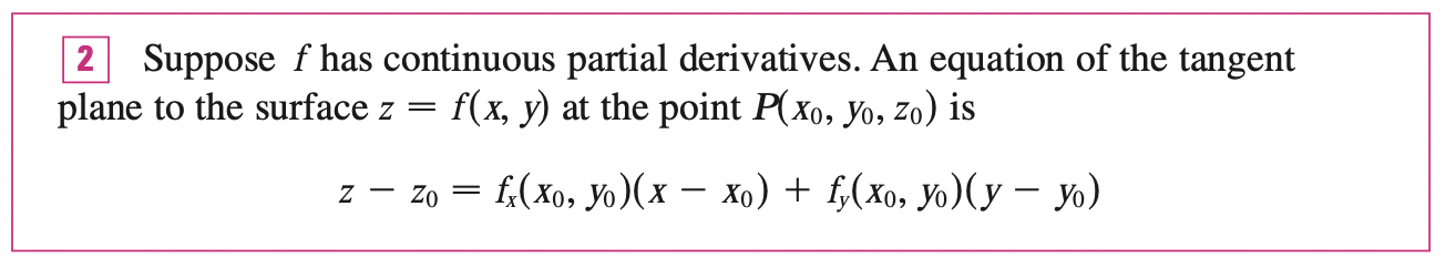
Suppose a surface \(S\) (the graph of \(f(x, y)\)) has equation \(z = f(x, y)\), where \(f\) has continuous first partial derivative, and let \(P(x_0, y_0, z_0)\) be a point on \(S\). Let \(C_1, C_2\) be the curves obtained by intersecting the vertical planes \(y=y_0, \; x=x_0\) (The curves are the graphs of \(f(x, y_0), \; f(x_0, y)\)). Let \(T_1, T_2\) be the tangent lines to the curves \(C_1, C_2\) at point \(P\). Then the slopes of these tangent lines are the partial derivatives (\(f_x, f_y\)) at point \(P\). Then the tagent plane to the surface \(S\) at the point \(P\) is defined to be the plane that contains both tangent lines \(T_1\) and \(T_2\).
If \(C\) is any other curve that lies on the surface \(S\) and passes through \(P\), then its tangent line at \(P\) also lies in the tangent plane (plane contains of all possible tangent lies at \(P\) to curves that lie on \(S\) and pass through \(P\)). The tangent plane at \(P\) is the plane that most closely approximates the surface \(S\) near the point \(P\).
We know that any plane passing through the point \(P(x_0, y_0, z_0)\) has an equation of the form:
\[A(x - x_0) + B(y - y_0) + C(z - z_0) = 0\]
By dividing this equation by \(C\) and letting \(a = -\frac{A}{C}, \; b = -\frac{B}{C}\), we can rewrite:
\[z - z_0 = a(x - x_0) + b(y - y_0)\]
Then the intersection between the plane \(y = y_0\) and the tangent plane at point \(P\) must be the tangent line \(T_2\) (\(y = y_0\)):
\[z - z_0 = a(x - x_0)\]
We know that this is the equation of tangent line \(C_2\) with slope \(a\), at the same time, we know that the slopes of this tangent line is the partial derivative at point \(P\):
\[a = f_x(x_0, y_0)\]
Similiar for \(C_1\), we have:
\[b = f_y(x_0, y_0)\]
Linear Approximation
We know that the equation of the tangent plane to the graph of function \(f(x, y)\) at point \(P\) is:
\[z - z_0 = f_x(x_0, y_0) (x - x_0) + f_y(x_0, y_0) (y - y_0) \implies z - z_0 = f_x(x_0, y_0) (x - x_0) + f_y(x_0, y_0) (y - y_0) + f(x_0, y_0)\]
The linear function whose graph is the tangent plant, namely:
\[L(x, y) = f_x(x_0, y_0) (x - x_0) + f_y(x_0, y_0) (y - y_0) + f(x_0, y_0)\]
is called the lineariation of \(f\) at \((x_0, y_0)\) and the approximation at point \((x_0, y_0)\)
\[L(x, y) \approx f(x, y)\]
is called linear approximation of \(f\) at point \((x_0, y_0)\).
Differentials
For a differentiable function of one variable \(y = f(x)\), we define the differential \(dx\) to be an independent variable, that is, \(dx\) can be given the value of any real number. The differential of y is then defined as:
\[dy = f^{\prime} (x)dx\]
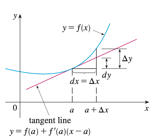
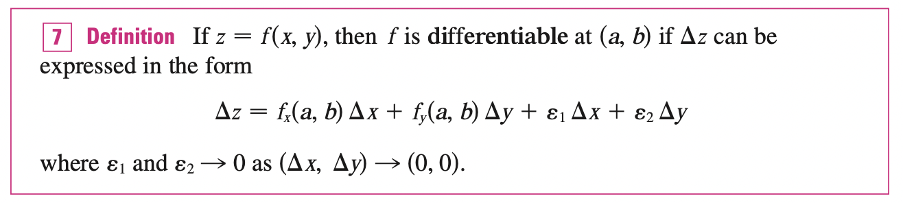
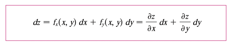
For a differentiable function of two variables \(z = f(x, y)\), we define the differentials \(dx,\; dy\) to be independent variables. Then the differential \(dz\) which is also called total differential is defined by:
We can rewrite the differential of \(z\) as the equation of tangent plane at point \(P\) to the graph of function \(f\) with
\[dz = \Delta z = z - z_0\] \[dy = \Delta y = y - y_0\] \[dx = \Delta x = x - x_0\]
Thus, the linear approximation equation can be rewrite in terms of differentials:
\[f(x, y) \approx z = f(a, b) + dz\]
Functions of Three or More Variables
Linear approximations, differentiability, and differentials can be defined in a similar manner for functions of more than two variables.
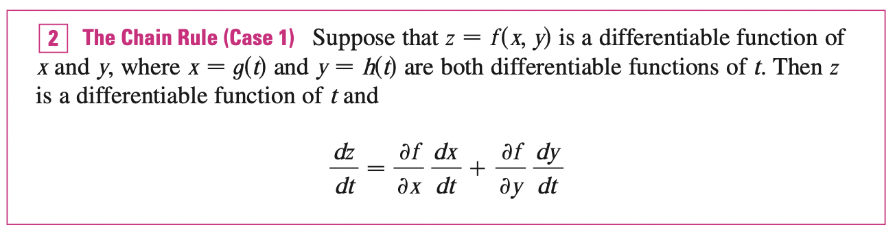
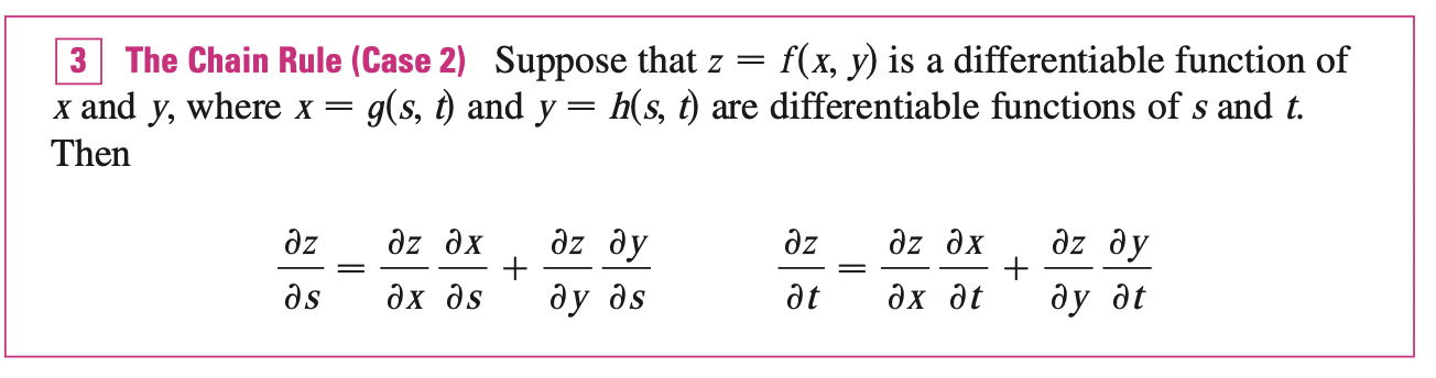
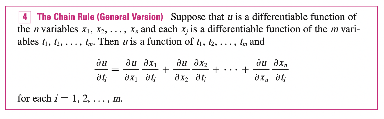
The Chain Rule
Implicit Differentiation
Suppose we have function of the form \(F(x, y) = 0, \forall x \in \mathbb{D}\), where \(y = f(x)\) is a function of \(x\). If \(F\) is differentiable, \(\frac{\partial F}{\partial y} \neq 0\), then:
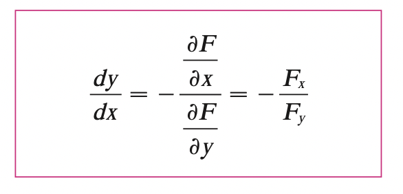
By Implicit Differentiation Theorem, this is valid only if:
- \(F\) is defined on a disk containing \((a, b)\), where \(F(a, b) = 0, \; F_y (a, b) \neq 0\)
- \(F_x, \; F_y\) is continuous on the disk
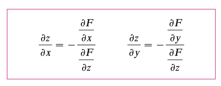
Also, if we have function defined \(f (x, y, z) = 0, \; z = f(x, y)\):
Directional Derivatives and the Gradient Vector
Directional Derivatives
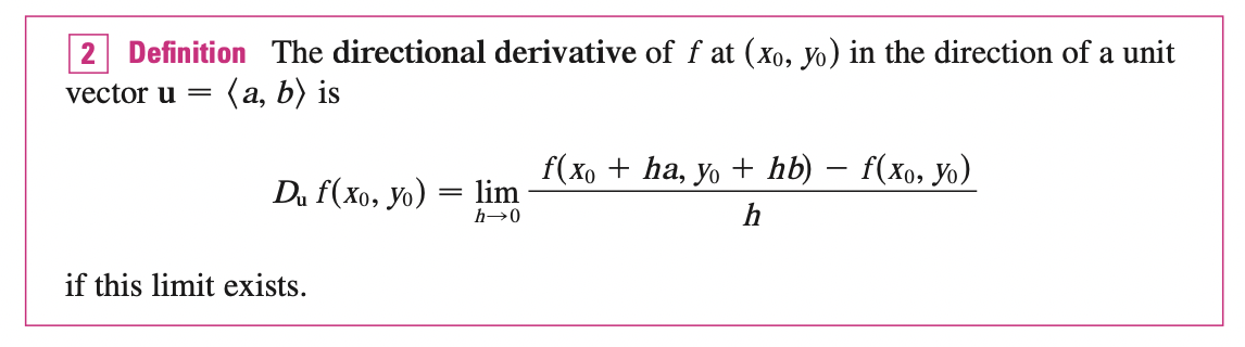
We know that the paritial derivatives represent the rates of change of \(z\) in the \(x, y\) directions, that is, in the direction of unit vectors \(i, j\). Suppose that we know wish to find the rate of change of \(z\) at \((x_0, y_0)\) in the direction of an arbitrary unit vector \(\mathbf{u} = <a, b>\).
To do this, we consider a surface \(S\) with equation \(z = f(x, y)\) (the graph of \(f\)) and we let \(z_0 = f(x_0, y_0)\), then the point \(P_0 (x_0, y_0, z_0)\) lies on the surface \(S\). The vertical plane that passes through \(P\) in the direction of \(\mathbf{u}\) intersects \(S\) in a curve \(C\). The slope of the tangent line \(T\) to \(C\) at point \(P\) is the rate of change of \(z\) in the direction of \(\mathbf{u}\)
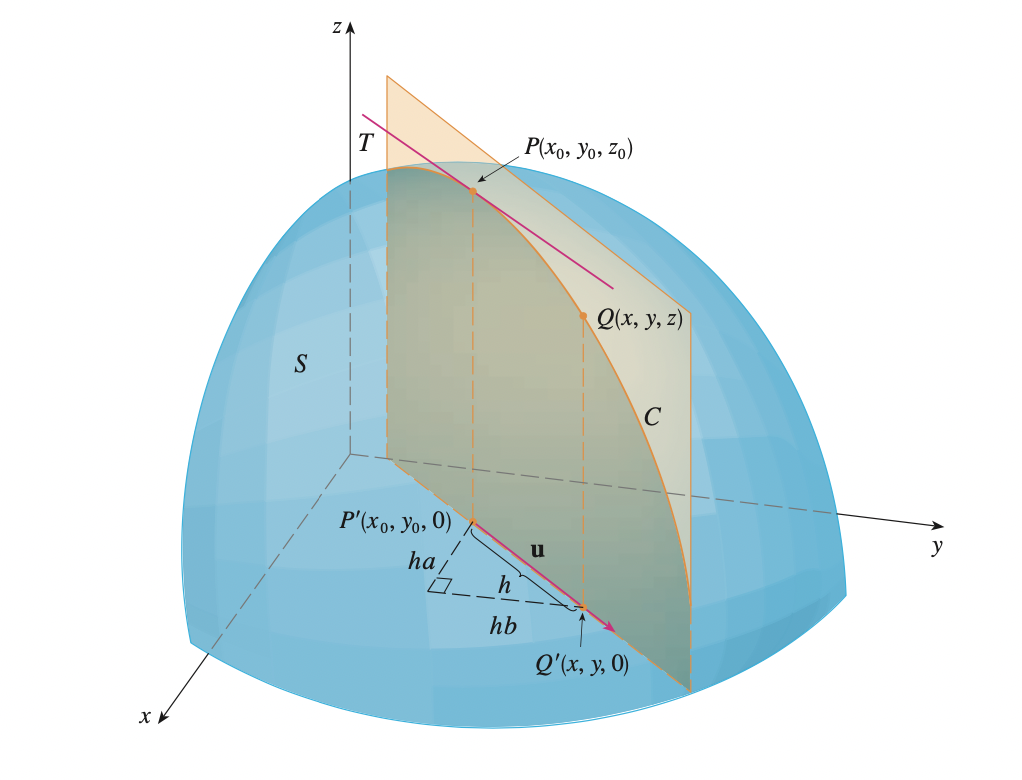
If \(Q(x, y, z)\) is another point on \(C\) and \(P^{\prime}, Q^{\prime}\) are the projections of \(P, Q\) onto the \(x, y\)-plane, then the vector \(\vec{P^{\prime}Q^{\prime}}\) is parallel to \(\mathbf{u}\) and:
\[\vec{P^{\prime}Q^{\prime}} = h \mathbf{u} = <ha, hb>\]
for some scalar \(h\). Therefore, \(\Delta x = x - x_0 = ha, \; \Delta y = y - y_0 = hb\):
\[\Delta z = z - z_0 = f(ha + x_0, hb + y_0) - f(x_0, y_0)\]
\[\frac{\Delta z}{h} = \frac{f(ha + x_0, hb + y_0) - f(x_0, y_0)}{h}\]
If we take limit to 0, we have the rate of change of \(z\) with respect to distance in the direction of \(\mathbf{u}\), we call this the directional derivative of \(f\) in the direction of \(\mathbf{u}\):
If we let \(\mathbf{u} = \mathbf{i} = <1, \;0>\), then we have \(D_i f = f_x\). If we let \(\mathbf{u} = \mathbf{j} = <0, \;1>\), then we have \(D_j f = f_y\). Partial derivatives are special cases of the directional derivative in the direction of x axis and y axis
The Gradient Vector
We can write the directional derivative formula as dot product:
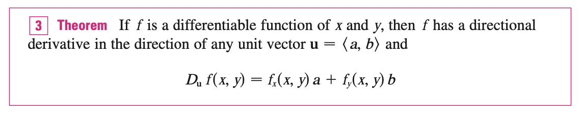
\[D_u f(x, y) = f_x(x, y)a + f_y(x, y)b = \; <f_x(x, y), \; f_y(x, y)> \cdot \; \mathbf{u}\]
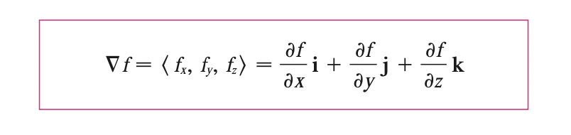
The first vector in the dot product is called the gradient of f
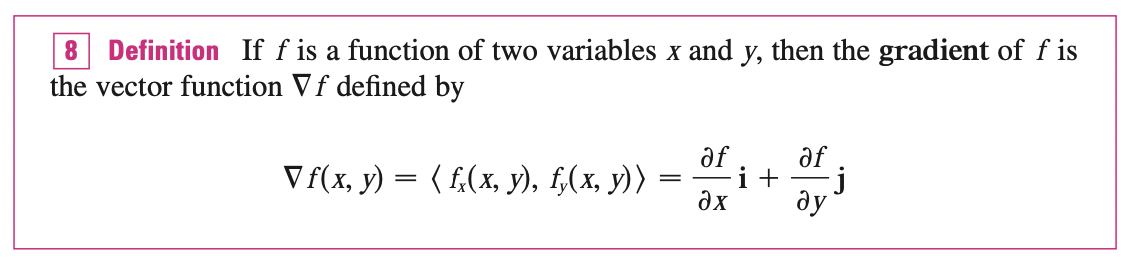
Recall that, the scalar projection \(comp_a b = \frac{a \cdot b}{|a|}\), so the directional derivative can be interpreted as the scalar projection of gradient vector onto the unit vector \(u\).
Functions of Three Variables
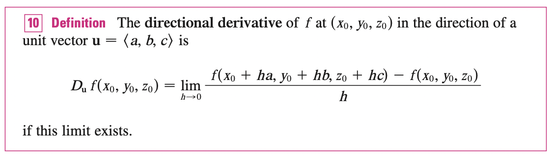
For functions of three variables, we can define directional derivatives similarly
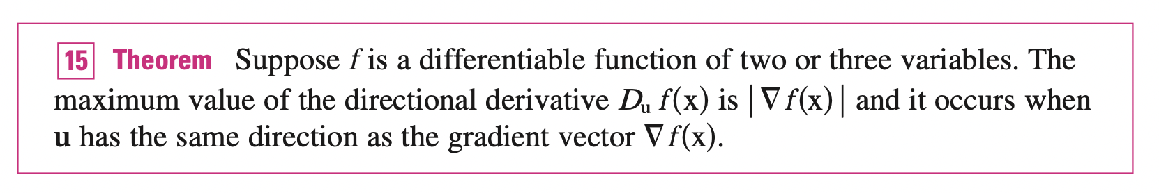
Maximizing the Directional Derivative
Suppose that we have a function \(f\) of two or three variables, and we consider all possible directional derivatives of \(f\) at a given point. These give the rates of change of \(f\) in all possible directions. What is the maximum rate of change?
Recall that:
\[D_{\mathbf{u}} f = \nabla f \cdot \; \mathbf{u} = |\nabla f||\mathbf{u}| \cos \theta\]
When \(\theta = 0\), \(cos \;\theta = 1\) and this is at its maximum. Thus:
\[\max D_{\mathbf{u}} f = |\nabla f|\]
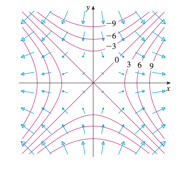
The maximum of the directional derivatives is the length of gradient vector at the direction of gradient vector. Since, the slope or rate of change is positive, we have steepest increase.
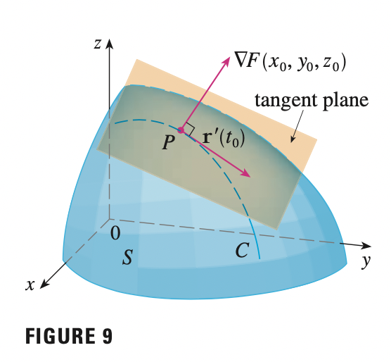
Tangent Planes to Level Surfaces
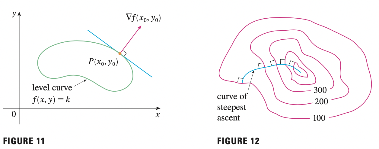
Suppose \(S\) is a surface with equation \(F(x, y, z) = k\), that is, it is a level surface of a function \(F\) of three variables, and let \(P(x_0, y_0, z_0)\) be a point on \(S\). Let \(C\) be any curve that lies on the surface \(S\) and passes through the point \(P\). Recall that, the curve is described by a vector function \(r(t) = <x(t), y(t), z(t)>\). Let \(t_0\) be the parameter value corresponding to \(P\). That is \(r(t_0) = P = <x_0, y_0, z_0>\). Since \(C\) lies on \(S\), any point \((x(t), y(t), z(t))\) must satisfy the equation of \(S\), that is:
\[F(x(t), y(t), z(t)) = k\]
If \(F, x, y, z\) is differentiable w.r.t \(t\):
\[\frac{dF}{dt} = \frac{\partial F \partial x}{\partial x \partial t} + \frac{\partial F \partial y}{\partial y \partial t} + \frac{\partial F \partial z}{\partial z \partial t} = 0\]
But, since \(\nabla F = <F_x, F_y, F_z>\) and \(r^{\prime} (t) = <x^{\prime} (t), y^{\prime} (t), z^{\prime} (t)>\), we can rewrite the above equation as:
\[\nabla F \cdot r^{\prime} (t) = 0\]
Thus, \(\nabla F\) is orthogonal to the tangent vector \(r^{\prime} (t)\), in particular at point \(P\):
\[\nabla F(x_0, y_0, z_0) \cdot r^{\prime} (t_0) = 0\]
So, if \(\nabla F(x_0, y_0, z_0) \neq 0\), it is natural to define the tangent plane to the level surface \(F(x, y, z) = k\) at \(P(x_0, y_0, z_0)\) as the plane that pass through \(P\) that has normal vector \(\nabla F(x_0, y_0, z_0)\). Using the standard equation of a plane, we have:
\[F_x(x_0, y_0, z_0) (x - x_0) + F_y (x_0, y_0, z_0) (y - y_0) + F_z (x_0, y_0, z_0) (z - z_0) = 0\]
The normal line to \(S\) at \(P\) is the line passing through \(P\) and perpendicular to the tangent plane. The direction of the normal line is therefore given by the gradient vector \(\nabla F(x_0, y_0, z_0)\).
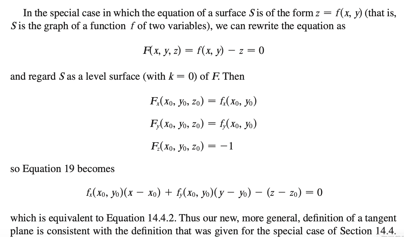
Note that, the tangent plane equation for function of two variables can be derived from this more general form of equation:
Maximum and Minimum Values
If the inequalities in definition 1 hold for all points \((x, y)\) in the domain of \(f\), then \(f\) has an absolute maximum or absolute minimumat \((a, b)\).
If \(f_x(a, b) = 0, \; f_y (a, b) = 0\), then the tangent plane at point \((a, b)\) is:
\[f_x(a, b) (x - a) + f_y (a, b) (y - b) - (z - z_0) = 0 \implies z = z_0\]
Thus, if \(f\) has a local maximum or minimum at point \((a, b)\), then the tangent plane at this point on the graph must be horizontal (\(z = z_0\)).
This point \((a, b)\) is called critical point or stationary point of \(f\) if \(f_x(a, b) = 0, \; f_y (a, b) = 0\) (has gradient 0) or if one of these partial derivatives does not exist. All local maximum and minimum are critical points, however, not all critical points are local maximum or minimum.
Example:
Consider the example \(f(x, y) = y^2 - x^2\), then \(f_x = -2x, \; f_y = 2y\). This implies there is only one critical point \((0, 0)\) for function \(f\). We compute \(x > 0\) for \(y = 0\), we have \(f(x, y) < 0\). If we compute \(y > 0\) for \(x = 0\), we have \(f(x, y) > 0\). Thus, we do not have a minimum, or a maximum at this critical point.
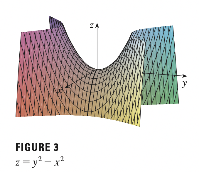
In this case, we have maximum in the direction of \(x\) but minimum in the direction of \(y\), thus, we have a saddle point at \((0, 0)\).
In order to distinguish between critical points, we can use second derivative test:
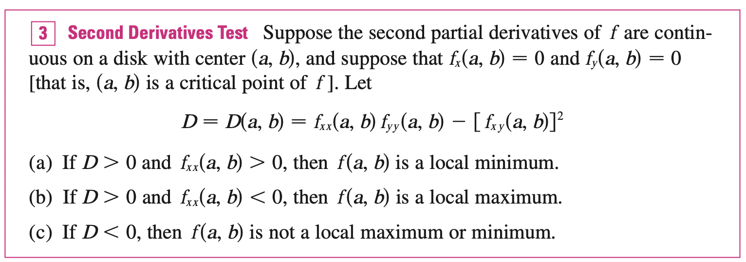
Notes:
- In case c, the point \((a, b)\) is the saddle point of \(f\) and the graph of \(f\) crosses its tangent plane at \((a, b)\).
- If \(D = 0\), the test is useless.
- \(D\) is actually the determinant of the Hessian matrix
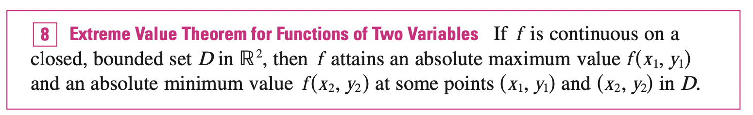
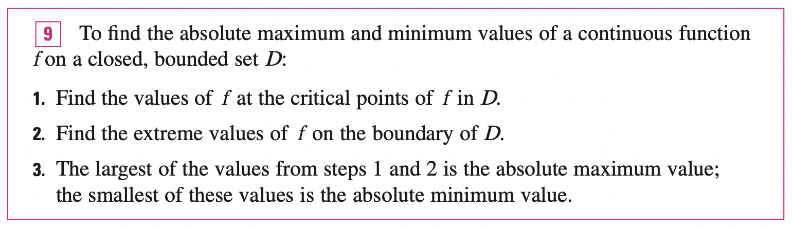
Absolute Maximum and Minimum Values
A bounded set in \(\mathbb{R}^2\) is one that is contained within some disk (less than and greater than some real numbers). In other words, it is finite in extent. A close set in \(\mathbb{R}^2\) is one that contains all its boundary points.
Lagrange Multipliers
Lagrange's method is used for maximizing or minimizing a general function \(f(x, y, z)\) subject to a constraint of the form \(g(x, y, z) = k\). We start by considering function of two variables, \(f(x, y)\) subject to constraint \(g(x, y) = k\). Recall that \(g(x, y) = k\) is a level curve, that is we can think of the optimization problem as finding the extreme value of \(f(x, y)\) when the points \((x, y)\) are restricted on the level curve \(g(x, y) = k\). It is also equivalent to find the largest value of \(c\) s.t the level curve \(f(x, y)=c\) intersects with the level curve \(g(x, y) = k\). That is, when they have common tangent line and their gradient vectors are parallel:
\[\nabla f(x_0, y_0) = \lambda \nabla g(x_0, y_0)\]
This kind of argument also applies to the problem of finding the extreme values of \(f(x, y, z)\) subject to \(g(x, y, z) = k\). Thus, the point \((x, y, z)\) is restricted to lie on the level surface \(S\) with equation \(g(x, y, z) = k\).
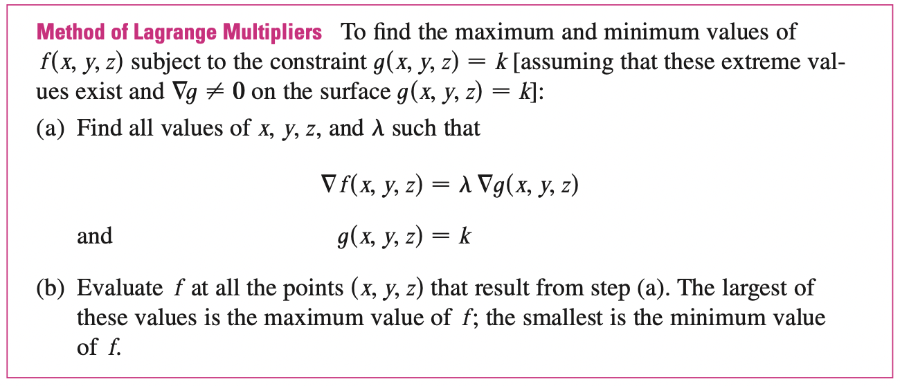
The number \(\lambda\) is called lagrange multiplier. We assume that \(\nabla g \neq 0\).
Two Constraints
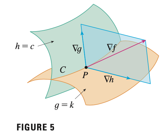
Suppose now we want to find the maximum and minimum values of a function \(f(x, y, z)\) subject to two constraints \(g(x, y, z) = k, h(x, y, z) = c\). Geometrically, this means that we are looking for the extreme values of \(f\) when \((x, y, z)\) is restricted to lie on the curve of intersection \(C\) of the level surfaces \(g(x, y, z) = k\) and \(h(x, y, z) = c\).