Monte Carlo Estimation

Learning From Stream of Data (Monte Carlo Methods)

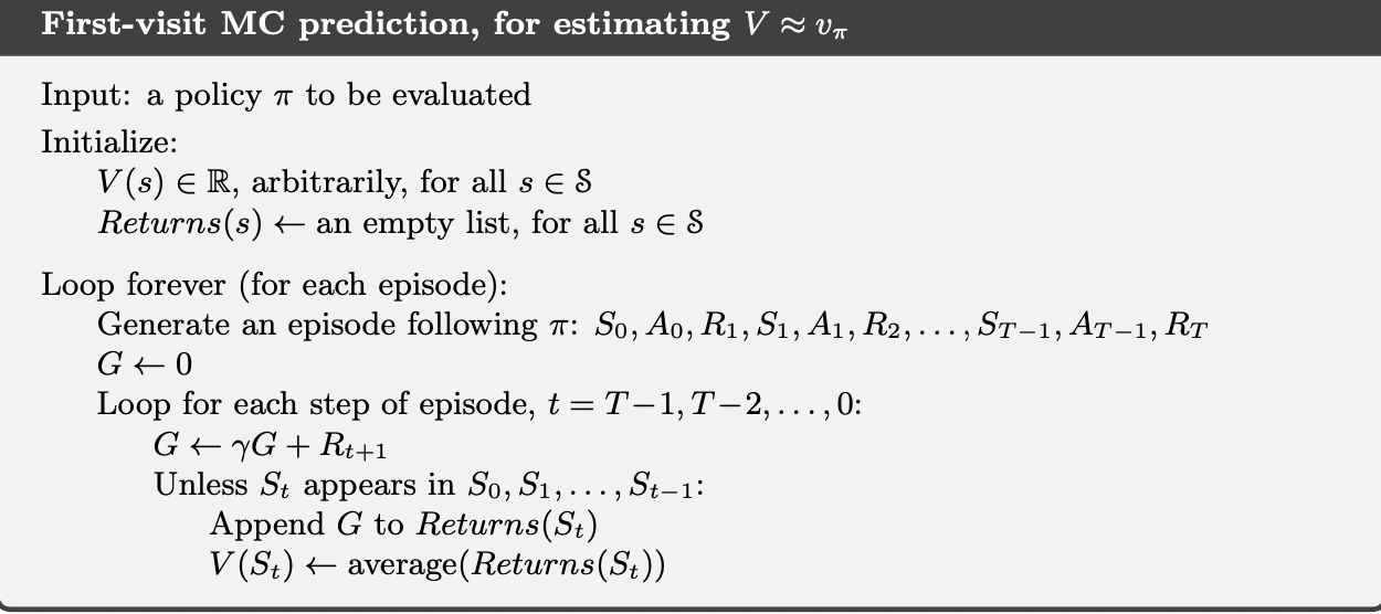
MC Policy Evaluation

The Goal is to learn or estimate the value function \(V^{\pi}\) and \(Q^{\pi}\) of a policy.

Recall that:

\[V^{\pi}(x) = E[G^{\pi}_{t} | X_t=x]\]

This is the expected return starting from state \(x\). At the same time, obtain a sample from return \(G^{\pi}\) is easy: if the agent starts at state \(x\), and follows \(\pi\), we can draw one sample of r.v \(G^{\pi}\) by computing the cumulative sum of rewards collected during the episode starting from the state \(x\):

\[\hat{G^{\pi}_{t}} = \sum^{\infty}_{k=t} \gamma^{k-t} R_{k}\]

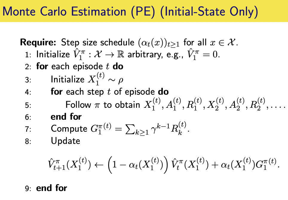
If we repeat this process from the same state, we get another draw of r.v \(G^{\pi}\), let us call these samples \(G^{\pi (1)} (x)\), \(G^{\pi (2)} (x)\), ...., \(G^{\pi (n)} (x)\). We can get an estimate \(\hat{V^{\pi}} (x)\) of \(V^{\pi} (x)\) by taking the average of the sample average:

\[\hat{V^{\pi}} (x) = \frac{1}{n} \sum^{n}_{i=1} \hat{G}^{\pi(i)} (x)\]

This follows by the weak law of large number, we can also estimate this expectation using Stochastic Approximation (SA) procedure to obtain an online fashion update:

\[ \hat{V^{\pi}_{t+1}} (x) \leftarrow (1 - \alpha_t) \hat{V^{\pi}_{t}} (x) + \alpha_t G^{\pi (t)} (x)\]

First Visit and Every Visit MC

Above two algorithms are examples of first visit MC method. Each occurrence of state \(x\) in an episode is called a visit to \(x\). Of course, \(x\) may be visited multiple times in the same episode; let us call the first time it is visited in an episode the first visit to \(x\). The first-visit MC method estimates \(V^{\pi} (x)\) as the average of the returns following first visits to \(x\), whereas the every-visit MC method averages the returns following all visits to \(x\).

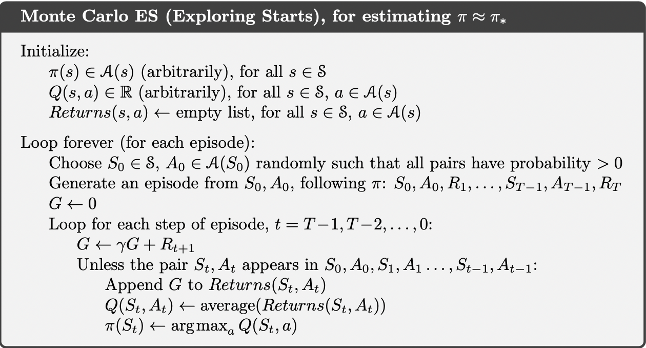
MC Control

Exploring Start

The general idea of MC control is to use some version of Policy Iteration. If we run many rollouts from each state-action pair \((x, a)\), we can define \(\hat{Q^{\pi}_t}\) that converges to \(Q^{\pi}\). If we wait for an infinite time:

\[Q^{\pi}_{\infty} = lim_{t \rightarrow \infty} \hat{Q^{\pi}_{t}} = Q^{\pi}\]

We can then choose:

\[\pi^{\prime} \rightarrow \pi_g (\hat{Q^{\pi}_{\infty}})\]

Then we repeat this process until convergence.

However, we do not need to have a very accurate estimation of \(Q^{\pi_k}\) before performing the policy improvement step. We can perform MC for a finite number of rollouts from each state, and then perform the improvement step. The below algorithms are MC control with Exploring Start, which assumes that for every state action pairs \((x, a)\), we have positive probability that we start at this state action pair.

or online version using exploring start:

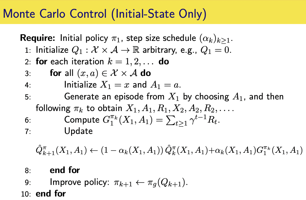
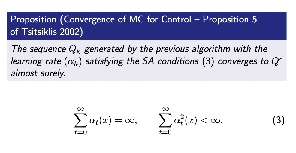
We can see that all returns are cumulated and averaged irrespective which policy they follow, however, the algorithm can still converge to \(Q^{*}\):

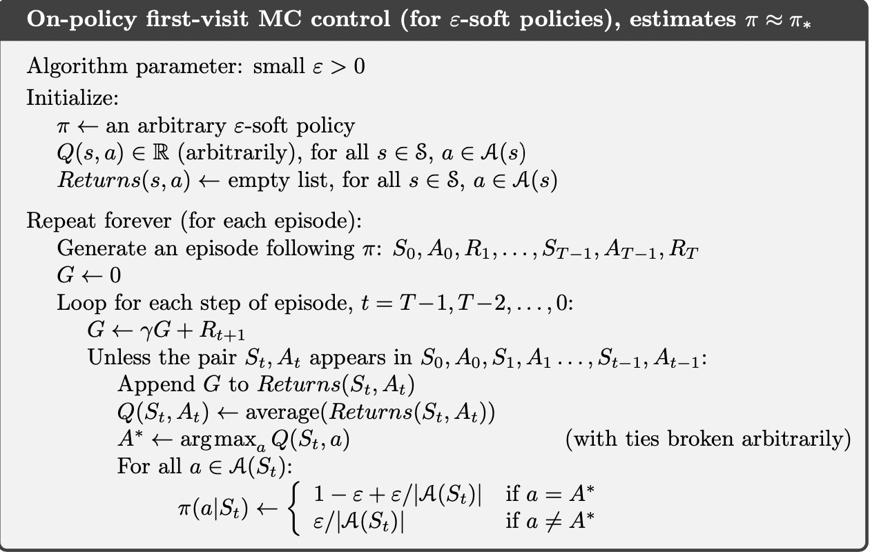
Without Exploring Start

Even though we are guaranteed to converge optimal action value function using MC with exploring start, however, this assumption of exploring start is unlike especially when state space and action space are large. To avoid this unlikely assumption, we can replace exploring start with \(\epsilon\)-soft policies to ensure sufficient exploration or using off-policy algorithms.

Further

In this post, we have some basic understanding of generic MC methods and basic framework of MC Policy evaluation and control. Next, we will explore some popular MC methods for solving control problems. We will see that MC methods can be generalized to both on-policy sampling scenario and off-policy sampling scenario.