Temporal Difference Learning

Learning From Stream of Data (Temporal Difference Learning Methods)

We can see that from MC algorithm, in order to update \(\hat{Q^{\pi}}_{k+1} (x, a)\), we need to calculate the entire \(\hat{G^{\pi}_{k}}\) which involves sum over product of rewards. If each episode is long or even continuous, the calculation of \(\hat{G^{\pi}_{k}}\) will be hard or impossible. In general, MC is agnostic to the MDP structure, if the problem is an MDP, it does not benefit from the recursive property of the value functions.

TD methods benefit from the structure of the MDP even if we do not know the environment dynamics \(P\) and \(R\).

TD for Policy Evaluation

We first focus on VI for PE: at each state \(x\), the procedure is:

\[V_{k+1} (x) = T^{\pi} V_{k} (x) = r^{\pi} (x) + \gamma \int P(dx^{\prime} | x, a) \pi(da | x) V_{k} (x^{\prime})\]

If we do not know \(r^{\pi}, P\), we cannot compute this. Suppose that we have n samples starting from state \(x\), \(A_i \sim \pi(\cdot | x), X^{\prime}_i \sim P(\cdot | x, A_i), R_i \sim R(\cdot | x, A_i)\), using these samples and \(V_{k}\), we compute:

\[Y_i = R_i + \gamma V_{k} (X_i^{\prime})\]

Now, notice that:

\[E[R_i | X=x] = r^{\pi} (x)\]

and

\[E[V_{k} (X^{\prime}_i) | X=x] = \int P(dx^{\prime} | x, a) \pi(da | x)V_{k} (x^{\prime})\]

so the r.v $Y_i (x) $ (emphasis starting from state \(x\) )satisfies:

\[E[Y_i | X=x] = E[R_i + \gamma V_{k} (X_i^{\prime}) | X=x] = E[R_i | X=x] + \gamma E[V_{k} (X_i^{\prime}) | X=x] = T^{\pi} V_{k} (x)\]

This implies that \(Y_i\) is an unbiased estimator of \(T^{\pi} V_{k}\) evaluated at \(x\). Thus, we can use a sample mean of \(Y_i\) starting from \(x\) to estimate \(T^{\pi} V_k (x)\), or we can use SA procedure.

\[T^{\pi}V^{t+1}_{k} (x) \leftarrow (1 - \alpha_t) T^{\pi}V^{t}_{k} (x) + \alpha Y_i\]

Empirical Bellman Operator

This \(Y_i\) is called empirical Bellman operator (this (x) notation emphasises that we are starting from x):

\[\hat{T}^{\pi} V_{k} (x) = Y_i (x) = R(x) + \gamma V_{k} (X^{\prime} (x))\]

This operator is an unbiased estimate of \(T^{\pi} V_{k} (x)\):

\[E[\hat{T}^{\pi} V_k (X) | X=x] = T^{\pi} V_{k} (x)\]

The empirical version of the VI for Policy evaluation with some noise:

\[V_{k+1} (x) \leftarrow \hat{T}^{\pi} V_k (x) = \underbrace{T^{\pi} V_{k} (x)}_{\text{deterministic part}} + \underbrace{(\hat{T}^{\pi} V_k (x) - T^{\pi} V_{k} (x))}_{\text{the stochastic part, the noise}}\]

On average, this noise is 0.

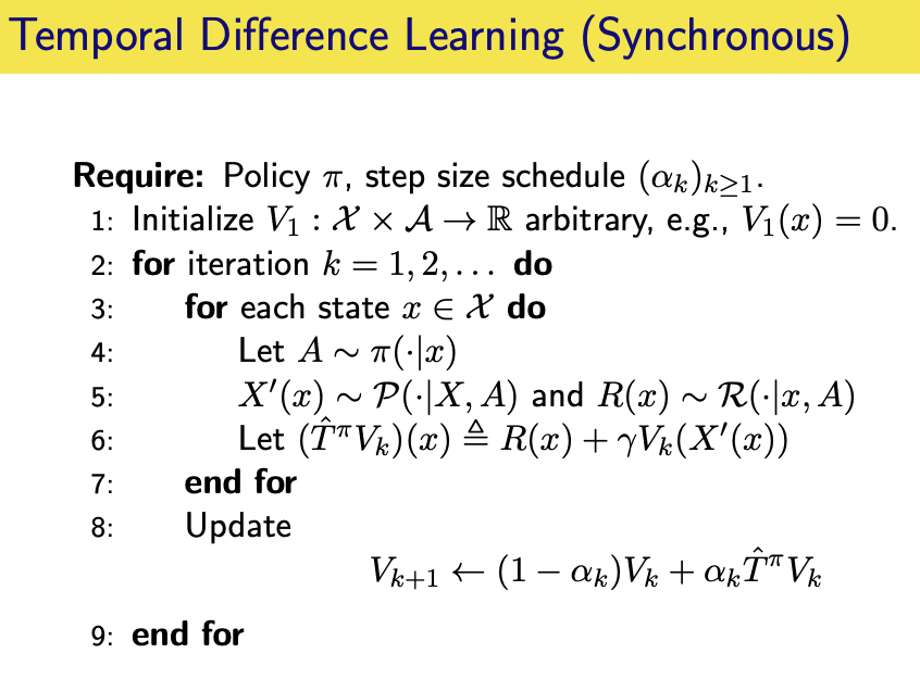
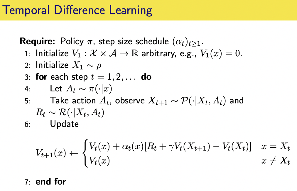
Generic TD algorithms

A synchronous version of generic TD algorithm updates all states at the same time:

However, we do not need to update all states at the same time, an asynchronous version of generic TD algorithm:

From the above generic algorithms, we can see that the update following policy \(\pi\) in general is :

\[\begin{aligned} V_{t+1} (x) &\leftarrow (1 - \alpha_t) V_t (x) + \alpha_t (\hat{T}^{\pi} V_t (x)) \\ &\leftarrow (1 - \alpha_t) V_t (x) + \alpha_t (R(x) + \gamma V_t (X^{\prime} (x)))\\ &\leftarrow V_t (x) + \alpha_t (x) [R_t (x) + \gamma V_t(X^{\prime} (x)) - V_t (x)] \end{aligned}\]

The update rule could be written in perhaps a simpler but less precise, form of:

\[V(X_t) \leftarrow V(X_t) + \alpha_t (X_t) [R_t + \gamma V(X_{t+1}) - V(X_t)]\]

We can see that, at each time step, instead update \(V_{k+1} (x)\) with \(T^{\pi} V_{k}\), we update it with the empirical bellman operator \(\hat{T}^{\pi} V_k\) which is an unbiased estimate. The SA procedure seems a little strange because we are estimating the mean of a sequence of \(\hat{T}^{\pi} V_1, \hat{T}^{\pi} V_2, ...\), we will prove later that this update rule actually converge to \(V^{\pi}\).

TD Error

TD Erorr and Bellman Residual

Moreover, the term:

\[\delta_t = R_t + \gamma V(X_{t+1}) - V(X_t)\]

is called TD error. It is a noisy measure of how close we are to \(V^{\pi}\). To see this more clearly, let us define the dependence on the TD error on its components more explicitly. Given transitions \((X, X^{\prime}, R)\) and value function \(V\), policy \(\pi\), we define:

\[\delta (R, X^{\prime}, X; V, \pi) = R + \gamma V(X^{\prime}) - V(X)\]

We have:

\[E[\delta (X, R, X^{\prime}; V, \pi) | X=x] = T^{\pi} V (x) - V(x) = BR(V) (x)\]

So in expectation, the TD error is equal to the Bellman residual of \(V\), evaluated at state \(x\). If BR = 0, we reach the fix point, so the algorithm reach the fix point.

TD Erorr and Advantage

The advantage function is defined as:

\[A^{\pi}(x, a) = Q^{\pi} (x, a) - V^{\pi} (x)\]

In expectation:

\[\begin{aligned} E[\delta (X, R, X^{\prime}; V^{\pi}) | X=x, A=a] &= E[R + \gamma V^{\pi}(X^{\prime}) - V^{\pi}(X) | X=x, A=a]\\ &= r(x, a) + \gamma \int_{x^{\prime}, a^{\prime}} P(x^{\prime} | x, a) \pi(a^{\prime} | x^{\prime})Q^{\pi} (x^{\prime}, a^{\prime}) - V^{\pi}(x)\\ &= Q^{\pi} (x, a) - V^{\pi} (x) \end{aligned}\]

Thus, the true TD error is an unbiased estimator of the advantage function.

TD Learning for Action-Value Function

We can use a similar procedure to estimate the action-value function which is often used in TD and MC.

To evaluate \(\pi\), we need to have an estimate of \(T^{\pi} Q (x, a) \forall (x, a) \in X \times A\).

Suppose that \((X_t, A_t) \sim \mu\) (where \(\mu\) is some stationary distribution or initial distribution) and \(X^{\prime}_t \sim P(\cdot | X_t, A_t)\) and \(R_t \sim R(\cdot | X_t, A_t), A^{\prime} \sim \pi(\cdot | X^{\prime})\)

The update rule would be:

\[Q_{t+1} (X_t, A_t) \leftarrow Q_t(X_t, A_t) + \alpha_t (X_t, A_t) [R_t + \gamma Q_t (X^{\prime}_t, A^{\prime}) - Q_t(X_t, A_t)]\]

and

\[Q_{t+1} (x, a) \leftarrow Q_t (x, a)\]

for all other \((x, a) \neq (X_t, A_t)\)

It is easy to see that following the same procedure for \(\hat{T}^{\pi} V\):

\[E[\hat{T}^{\pi} Q (X_t, A_t) | X_t=x, A_t=a] = T^{\pi} Q (x, a)\]

Further

In this post, we have some basic understanding of generic TD methods and basic framework of TD Policy evaluation. Next, we will explore some popular TD methods for solving control problems. We will see that TD learning methods can be generalized to both on-policy sampling scenario (ie. SARSA) and off-policy sampling scenario (ie. Q-learning). At the same time, we will prove the update rule for each algorithm.