Q-Learning

Temporal Difference Learning for Control: Q-Learning

We can use TD-like methods for the problem of control too. Consider any \(Q\). Let \(X^{\prime} \sim P(\cdot | X, A)\) and \(R \sim R(\cdot | X, A)\) and define:

\[Y = R + \gamma max_{a^{\prime} \in A} Q(X^{\prime}, a^{\prime})\]

We have:

\[E[Y | X=x, A=a] = r(x, a) + \gamma \int P(dx^{\prime} | x, a) max_{a^{\prime} \in A} Q(x^{\prime}, a^{\prime}) = T^{*} Q (x, a)\]

So, \(Y\) is an unbiased estimate of \(T^{*} Q (x, a)\). Let's define the empirical Bellman optimality operator \(\hat{T}^{*} Q (x, a)\):

\[T^{*} Q (x, a) = Y = R + \gamma max_{a^{\prime} \in A} Q(X^{\prime}, a^{\prime})\]

We can write the SA update rule for estimating \(Q^{*}\) as:

\[Q_{t+1} (X_t, A_t) \leftarrow Q_t(X_t, A_t) + \alpha_t (X_t, A_t) [R_t + \gamma max_{a^{\prime} \in A} Q_t (X^{\prime}_t, a^{\prime}) - Q_t(X_t, A_t)]\]

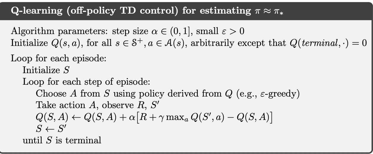
We can clearly see that Q-learning is an off-policy method, because we are generating the episode using \(\pi\) which is usually an \(\epsilon\)-greedy policy. However, we are evaluating the greedy policy (in update rule, we select according to the greedy policy not \(\pi\) i.e \(a^{\prime}\) is not selected by \(\pi\)).

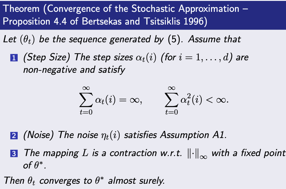
Proof: Convergence of Q-Learning

Suppose that we want to find the fixed-point of an operator \(L\):

\[L \theta = \theta\]

for \(\theta \in \mathbb{R}^{d}, L: \mathbb{R}^{d} \rightarrow \mathbb{R}^{d}\).

Consider the iterative update:

\[\theta_{t+1} \leftarrow (1 - \alpha) \theta_t + \alpha L\theta_t\]

\(L\theta_t\) can be anything such as \(T^{\pi} V_k\), as long as \(L\) is \(c-\)Lipschitz with \(c < 1\) and \(\alpha\) is small enough \((0 < \alpha < \frac{2}{1 - c})\), this would converge.

To see this, let:

\[L^{\prime}: \theta \rightarrow ((1 - \alpha) I + \alpha L) \theta\]

Then the above update rule can be rewritten as:

\[\theta_{t+1} \leftarrow L^{\prime} \theta_{t}\]

For any \(\theta_1, \theta_2 \in \mathbb{R}^{d}\), this new mapping satisfies:

\[\begin{aligned} \| L^{\prime} \theta_1 - L^{\prime}\theta_2 \| &= \|((1 - \alpha) I + \alpha L) \theta_1 - ((1 - \alpha) I + \alpha L) \theta_2\|\\ & \leq (1 - \alpha) \| \theta_1 - \theta_2 \| + \underbrace{\alpha \|L\theta_1 - L\theta_2 \|}_{\leq \alpha * c \| \theta_1 - \theta_2 \|} \\ & \leq ((1 - \alpha) + c \alpha) \| \theta_1 - \theta_2 \| \end{aligned}\]

If \((1 - \alpha) + c \alpha < 1 \implies 0 < \alpha < \frac{2}{1 - c}\), then \(L^{\prime}\) is a contraction mapping and by the Banach fixed point theorem, the iterative process converges.

However, in reality, we do not have access to \(L\theta_t\) in general, but only its noise contaminated version \(L\theta_t + \epsilon_t\) with \(\epsilon_t \in \mathbb{R}^{d}\) being a zero-mean noise, we have:

\[\theta_{t+1} \leftarrow (1 - \alpha_t) \theta_t + \alpha_t (L\theta_t + \epsilon_t)\]

Recall that \(\alpha_t\) can not be constant, otherwise the variance of the estimate would not go to zero. Assume that at time \(t\), the \(i\)-the component of \(\theta_t\) is updated as:

\[\theta_{t+1} (i) \leftarrow (1 - \alpha_t(i)) \theta_t(i) + \alpha_t(i) (L\theta_t(i) + \epsilon_t(i))\]

With \(\alpha_t (j) = 0, \forall j \neq i\) (other components are not updated)

Now, we know that this iterative process will converge, but which point will it converge?

Next, we will see that \(\theta_t\) converges to \(\theta^{*}\)

Convergence of \(\theta_t\) to \(\theta^{*}\)

Denote the history of the algorithm up to time \(t\) by \(F_t\):

\[F_t = \{\theta_0, ...., \theta_t\} \cup \underbrace{\{\epsilon_0, ...., \epsilon_{t-1}\}}_{\text{up to time t, the r.v } \epsilon_t \text{ is not observed}} \cup \{\alpha_0, ..., \alpha_t\}\]

We need more assumptions:

Assumption A1: 1. For every component \(i\) and time step \(t\), we have E[_t (i) | F_t] = 0 (we assume noise are i.i.d) 2. Given any norm \(\| \cdot \|\) on \(\mathbb{R}^{d}\), there exist constants \(c_1, c_2\) such that for all \(i, t\), we have:

\[\underbrace{E[|\epsilon_t (i) |^2 | F_t]}_{\text{variance of } \epsilon_t (i)} \leq c_1 + c_2 \| \theta_t \|^2\]

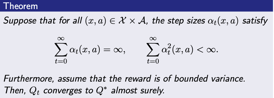
Convergence of \(Q_t\) to \(Q^{*}\)

The Q-learning update rule has the same form as the SA update rule:

• \(\theta\) is \(Q \in \mathbb{R}^{X \times A}\)
• the operator \(L\) is the bellman optimality operator \(T^{*}\)
• the index \(i\) in the SA update is the selected \((X_t, A_t)\)
• the noise term \(\epsilon_t (i)\) is the difference between \(\hat{T}^{*} Q - T^{*} Q\)

Suppose that at time \(t\), the agent is at state \(X_t\), takes action \(A_t\), gets \(X^{\prime}_t \sim P(\cdot | X_t, A_t), R_t \sim R(\cdot | X_t, A_t)\).

The update rule of the Q-learning is:

\[Q_{t+1} (X_t, A_t) \leftarrow (1 - \alpha_t(X_t, A_t))Q_t(X_t, A_t) + \alpha_t (X_t, A_t) [T^{*}Q_t (X_t, A_t) + \epsilon_t (X_t, A_t)]\]

with:

\[\epsilon_{t} (X_t, A_t) = R_t + \gamma max_{a^{\prime} \in A} Q_t (X^{\prime}_t, a^{\prime}) - T^{*} Q(X_t, A_t)\]

and:

\[Q_{t+1} (x, a) \leftarrow Q_t(x, a), \forall (x, a) \neq (X_t, A_t)\]

We know that:

• \(T^{*}\) is a \(\gamma\)-contraction mapping, so condition (3) of the Convergence of SA Theorem.
• Condition (1) of the Convergence of SA Theorem is assumed too.

We only need to verify condition (2) in order to apply the theorem.

Proof of Condition (2)

Let \(F_t\) be the history of algorithm up to and including when the step size #_t (X_t, A_t)$ is chosen, but just before \(X^{\prime}_t\) and \(R_t\) are revealed. This implies \(X_t=x, A_t=a\) is already given, but \(X^{\prime}_t, R_t\) are still unknown. We have:

\[E[\epsilon_t (X_t, A_t) | F_t] = E[R_t + \gamma max_{\alpha^{\prime} \in A} Q_t (X^{\prime}_t, a^{\prime}) | F_t] - E[T^{*} (Q_t) (X_t, A_t) | F_t] = 0\]

This verifies condition (a) of Assumption A1: zero-mean noise

To Verify (b) of Assumption A1, we provide an upper bound on \(E[\epsilon_t^2 (X_t, A_t) | F_t]\):

\[\begin{aligned} E[\epsilon_t^2 (X_t, A_t) | F_t] &= E[|(R_t - r(X_t, A_t)) + \gamma (max_{a^{\prime}} Q_t (X^{\prime}_t, a^{\prime}) - \int P(dx^{\prime} | X_t, A_t) Q_t (x^{\prime}_t, a^{\prime}))|^2 | F_t]\\ & \leq 2E[|(R_t - \underbrace{r(X_t, A_t)}_{E[R_t | X_t, A_t]})|^2 | F_t] + 2 E[|\gamma (max_{a^{\prime}} Q_t (X^{\prime}_t, a^{\prime}) - \underbrace{\int P(dx^{\prime} | X_t, A_t) Q_t (x^{\prime}_t, a^{\prime})}_{E[max_{a^{\prime} \in A} Q_t(X^\prime, a^{\prime})]})|^2 | F_t] \\ & \leq 2Var[R_t | X_t=x_t, A_t=a_t] + 2 \gamma^2 Var[max_{a^{\prime} \in A} Q_t (X^{\prime}, a^{\prime}) | X_t=x_t, A_t=a_t]\\ \end{aligned}\]

Thus:

\[\begin{aligned} Var[max_{a^{\prime} \in A} Q_t (X^{\prime}, a^{\prime}) | X_t=x_t, A_t=a_t] &= E[|max_{a^{\prime} \in A} Q_t (X^{\prime}, a^{\prime})|^2 | X_t=x_t, A_t=a_t] - E[max_{a^{\prime} \in A} Q_t (X^{\prime}, a^{\prime}) | X_t=x_t, A_t=a_t]^2\\ &\leq E[|max_{a^{\prime} \in A} Q_t (X^{\prime}, a^{\prime})|^2 | X_t=x_t, A_t=a_t]\\ &\leq max_{x, a} |Q^{t} (x, a)|^2 \\ &\leq \sum_{x, a} |Q_t(x, a)|^2 \text{ (i.e }max_x |f(x)| \leq \sum_x |f(x)|)\\ &= \| Q_t\|^2_2 \end{aligned}\]

Denote the maximum variance of the reward distributino over the state-action space \(max_{(x, a) \in X \times A} Var[R(x, a)]\) by \(\sigma^2_{R}\) which is assumed to be bounded, we have:

\[E[\epsilon_t^2 (X_t, A_t) | F_t] \leq 2 (\sigma^2_{R} + \gamma^2 \| Q_t\|^2_2)\]

Therefore, we can choose \(c_1 = 2\sigma^2, c_2 = 2\gamma^2\) in condition b of Assumption A1. All conditions of SA Convergence Theorem is satisfied, so Q_t converges to \(Q^{*}\)

Remark

• The step size condition is state-action dependent.
• If there is a state-action pair that is not selected at all or only a finite number of times, the condition cannot be satisfied. (ie. the sum does not go to infinity)
• We need each state-action pair to be visited infinitely often.
• The state-action-dependence of the step size might be different from how the Q-learning algorithm is sometimes presented, in which a single learning rate \(\alpha_t\) is used for all state-action pairs.
• A single learning rate suffices if the agent happens to visit all \((x, a) \in (X \times A)\) frequent enough.

Implementations: