Batch Normalization
Batch Normalization: Accelerating Deep Network Training by Reducing Internal Covariate Shift
Internal covariate shift describes the phenomenon in training DNN that the distribution of each layer's inputs changes during training, as the parameters of the previous layer change. This slow down the training by requiring lower learning rates and careful parameter initialization, and makes it notoriously hard to train models with saturating non-linearities (tanh, sigmoid). This problem can be addressed by normalizing the layer inputs.
Introduction
To see the input distribution shift in terms of sub-network or a layer. Consider a network computing:
\[l = F_2(F_1(\textbf{u}, \Theta_1), \Theta_2)\]
Where \(F_1\) and \(F_2\) are arbitrary transformations, and the parameters \(\Theta_1, \Theta_2\) are to be learned to minimize the loss \(l\). Learning \(\Theta_2\) can be viewed as if inputs \(\textbf{x} = F_1(\textbf{u}, \Theta_1)\) and fed into the sub-network:
\[l = F_2(\textbf{x}, \Theta_2)\]
Thus, a fixed input distribution (ie. the distribution of \(\textbf{x}\)) would make the training more effective, because \(\Theta_2\) does not need to adapt to the new distribution. At the same time, if the mapping \(F_2\) is saturating non-linearity, a fixed-distribution will help to prevent the gradient of parameters from vanishing.
Towards Reducing Internal Covariate Shift
Consider a layer with the input \(u\) that adds the learned bias \(b\), and normalizes the result by subtracting the mean of the activation computed over the training data \(\hat{x} = x - \bar{x}\), where \(\bar{x} = \frac{1}{N} \sum_{i=1}^{N} x_i\). If we ignore the dependence of \(b\) in \(\bar{x}\) (ie. \(\hat{x} = x - \mu\) we just center the input by some constant \(\mu\), does not take into account \(b\)), then
\[\frac{\partial L}{\partial b} = -\frac{\partial L}{\partial \hat{x}} \frac{\partial \hat{x}}{\partial b} = -\frac{\partial L}{\partial \hat{x}}\]
Then, the update rule is:
\[b \leftarrow b - \frac{1}{N}\sum_{i}\frac{\partial L}{\partial \hat{x}}\]
Let, \(\nabla b = - \frac{1}{N}\sum_{i}\frac{\partial L}{\partial \hat{x}}\) Then, new \(\hat{x}\) after update \(b\) is:
\[u + (b + \nabla b) + \frac{1}{N} \sum_i [u + (b + \nabla b)] = u + b - E[u + b]\]
Thus, the combination of the update to \(b\) and subsequent change in normalization led to no change in the output of the layer nor, consequently, the loss (ie. center the input without taking account of \(b\) will result useless update to \(b\) that has no effect on the loss). However, as the training continues, \(b\) will grow indefinitely while the loss remains the same.
This is caused because the gradient descent optimization does not take into account that the normalization takes place.
Normalization via Mini-Batch Statistics
Normalize the layer inputs are expensive, as it requires computing the covariance matrix, the inverse square root, the expectation over all training samples, as well as the derivative of these transformations. Several simplifications are proposed to deal with these.
Instead normalize the features in layer inputs and outputs jointly, we will normalize each scalar feature independently by making it have the mean of zero and the variance of 1. For a layer with \(d\)-dimensional input \(x = (x^{1}, ..., x^{d})\), we will normalize each individual feature:
\[\hat{x}^{k} = \frac{x^k - E[x^k]}{\sqrt{Var[x^k]}}\]
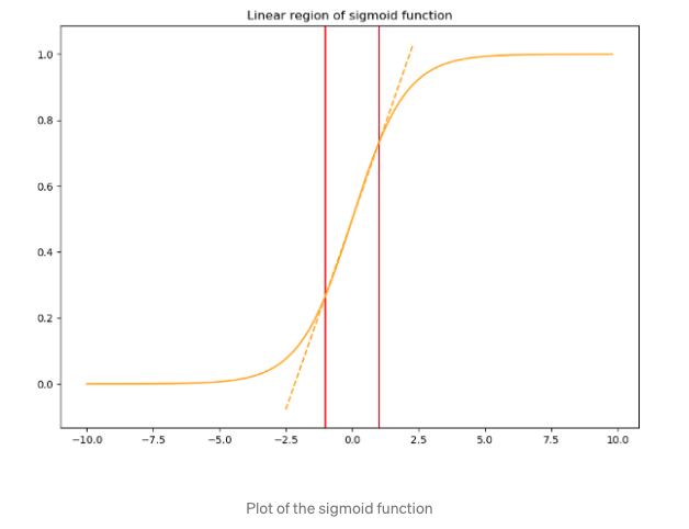
Where the expectation and variance are computed over the training dataset (i.e first input feature is normalized by first features of all input samples). However, this approach may decrease the expressive power of the activation function, for instance, if we scale the input of sigmoid activation to have mean 0 and variance 1, then we will be limited at the middle region of the sigmoid function (In this paper, batch norm is applied right after activation and before activation function)
To address this, we make sure that the transformation inserted in the network can represent the identity transformation, that is for each activation \(x^k\), a pair of parameters \(\gamma^k, \beta^k\), which scales and shift the normalized value:
\[y^k = \gamma^k \hat{x}^k + \beta^k\]
These parameters are learned through back propagation, and by setting \(\gamma^k = \sqrt{Var[x^k]}, \beta^k = E[x^k]\), we could recover the original activation, if that were the optimal thing to do.
- Instead of using whole batch of data for estimating mean and variance which is impractical in practice. We only use mini-batches to estimate means and variance, because mini-batches produce unbiased estimates of the mean and variance. Note that the use of mini-batches is enabled by computation of per-dimension variances rather than joint covariances (we do not estimate the covariance). In joint case, regularization would be required since the mini-batch size is likely to be smaller than the number of activations, resulting in singular covariance matrices.
Together, we can describe the batch norm transformation for each activation \(x\) as:
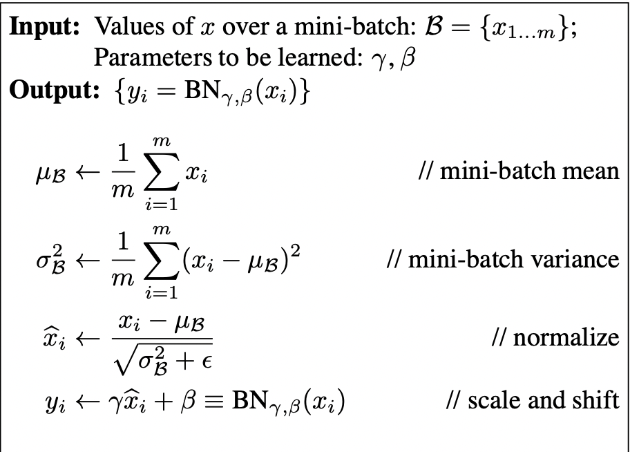
Where \(\epsilon\) is a constant added to the mini-batch variance for numerical stability, \(BN_{\gamma, \beta}: x_{1, ..., m} \rightarrow y_{1, ..., m}\) is the batch norm transformation. Since the normalization is applied to each activation independently, \(k\) which indicates the activation or dimension is dropped.
The backward pass can be write as:
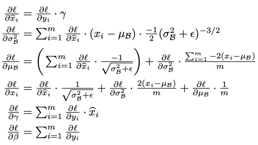
Notice that, \(\gamma, \beta\) have superscript \(k\), they bind to each activation.
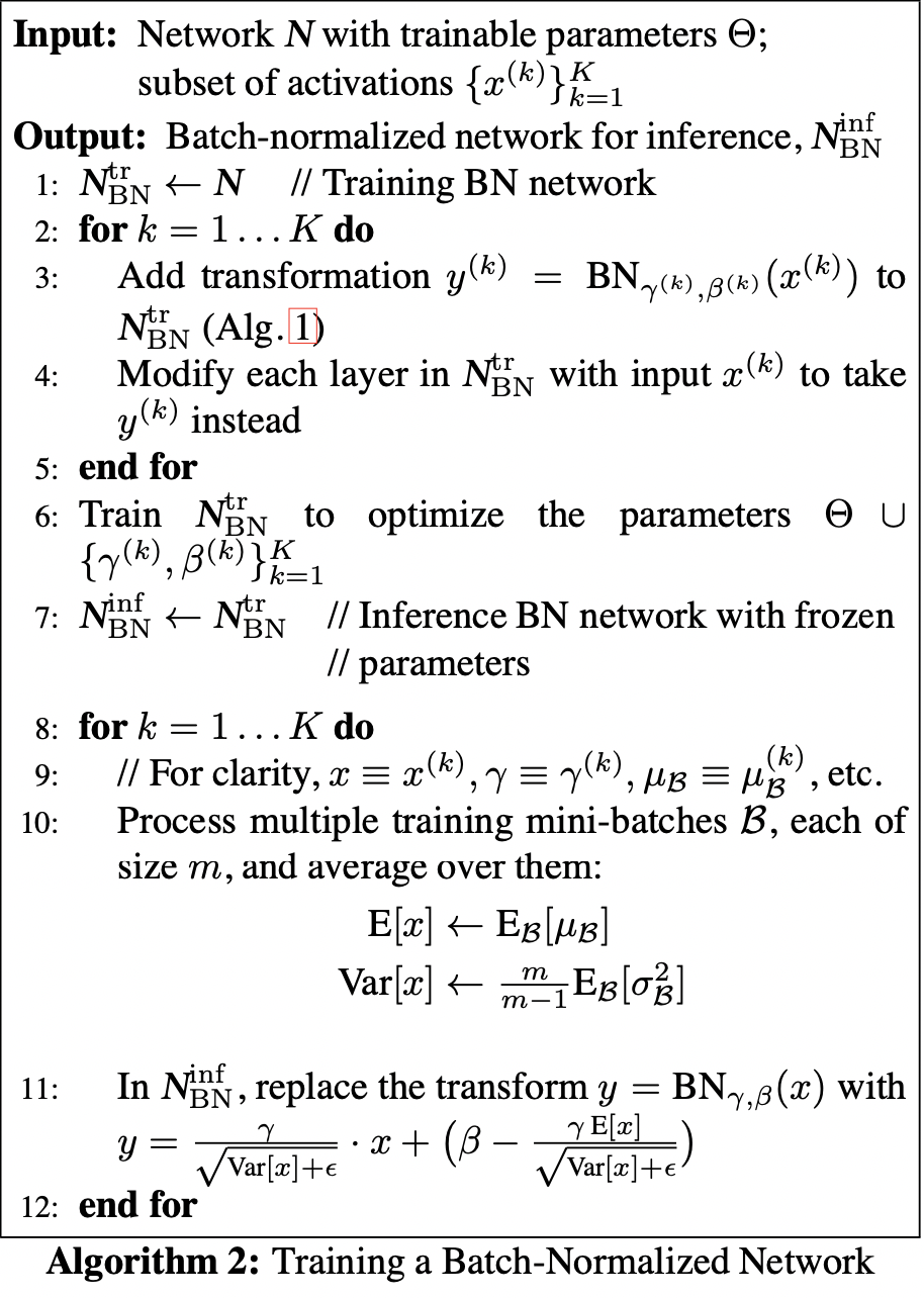
Training and Inference with Batch Normalized Network
To Batch-Normalize a network, any layer that previously received \(x\) as input now receive \(BN(x)\).
Training
A model employing Batch Normalization can be trained using batch gradient descent, or Stochastic Gradient Descent with a mini-batch size \(m > 1\) or any variant such as Adam. The normalization of activations that depends on the mini-batch allows efficient training. Using moving averages instead, we can track the accuracy of a model as it trains.
Testing
During testing, it is neither necessary nor desirable to estimate mean and variance using mini-batches, thus, once the network has been trained, we use the normalization:
\[\hat{x} = \frac{x - E[x]}{\sqrt{Var[x] - \epsilon}}\]
\[Var[x] = \frac{m}{m - 1} E_{B}[\sigma^2_{B}]\]
where \(E[x]\) is the mean for the whole dataset. The variance is a bias-corrected version of mini-batch sample variance over all training mini-batches weighted by their occurrence during training.
Batch Norm in Cov Net
For convolutional layers, we additionally want the normalization to obey the convolutional property ----- so that different elements of the same feature map, at different locations, are normalized in the same way (ie. features in the same feature are normalized in same way). So in the \(BN(x)\), we replace \(B\): mini-batch by \(B\): the set of all values in a feature map across both the elements of a mini-batch and spatial locations, for a mini-batch of size \(m\) and feature map of size \(p * q\) \(|B| = m * p * q\). We learn \(\gamma^k, \beta^k\) per feature map. So in total, we have \(C\) different means and variances, where \(C\) is number of input channels.
Side Effects of Batch Norm
With Batch Norm, back-propagation through a layer is unaffected by the scale of its parameters. \[ BN(\alpha W u) = BN(Wu) \] \[ \frac{\partial BN(\alpha Wu)}{\partial u} = \frac{\partial BN(Wu)}{\partial u}\] \[ \frac{\partial BN(\alpha Wu)}{\partial \alpha W} = \frac{1}{\alpha} \frac{\partial BN(Wu)}{\partial u}\]
Larger weights leads to smaller gradients, Batch Normalization stabilize the parameter growth:
\[\alpha = 100, \implies \frac{\partial BN(100 Wu)}{\partial 100 W} = \frac{1}{100} \frac{\partial BN(Wu)}{\partial u}\]
Use sample statistics from mini-batches introduce random noise, which helps with the overfitting.