Stochastic Graph
Gradient Estimation Using Stochastic Computation Graphs
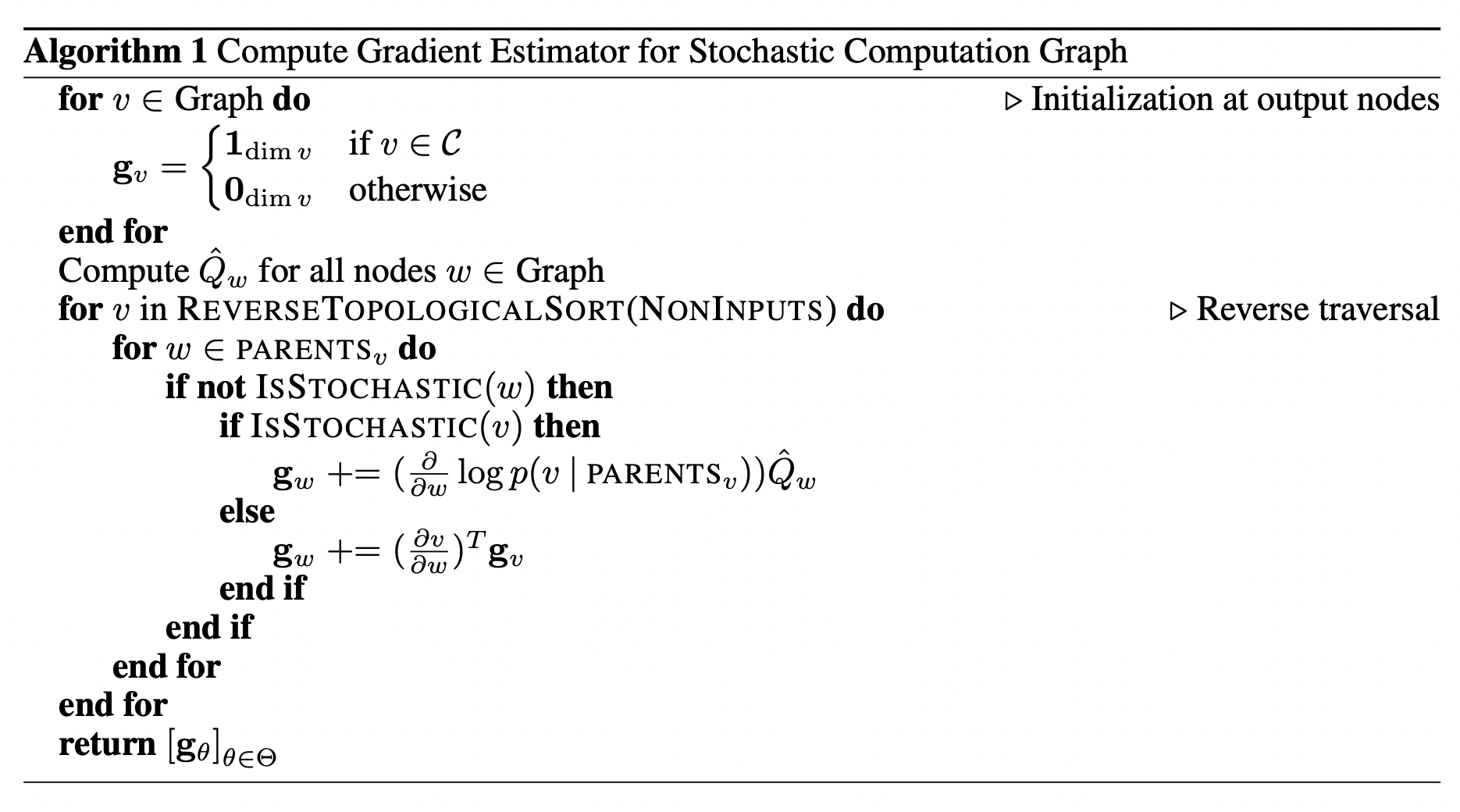
The backpropagation algorithm is only sufficient when the loss function is a deterministic, differentiable function of the parameter vector. The main practical result of this article is that to compute the gradient estimator, one just needs to make a simple modification to the backpropagation algorithm, where extra gradient signals are introduced at the stochastic nodes.
Preliminaries
Gradient Estimators for a Single Random Variable
Suppose \(X\) is a random variable, \(f\) is a function, we are interested in computing
\[\frac{\partial}{\partial \theta} E_{X}[f(X)]\]
There are few different ways that the process for generating \(X\) could be parameterized in terms of \(\theta\), which lead to different gradient estimators.
We might be given a parameterized probability distribution \(X \sim p(\cdot ; \theta)\). In this case, we can use score function or REINFORCE or likelihood ratio estimator estimator:
\[\frac{\partial}{\partial \theta} E_{X \sim p(\cdot ; \theta)}[f(X)] = \int_x \frac{\frac{\partial}{\partial\theta} p(x; \theta)}{p(x; \theta)} p(x; \theta) f(x)dx = E_{X \sim p(\cdot ; \theta)}[f(X) \frac{\partial}{\partial\theta} log p(X; \theta)]\]
This equation is valid if \(p(x; \theta)\) is a continuous function of \(\theta\); however it does not need to be a continuous function of \(x\)
\(X\) may be a deterministic, continuous function of \(\theta\) and another random variable \(Z\), we can write as \(X(\theta, Z)\). Then we can use the pathwise derivative or stochastic backpropagation estimator:
\[E_{Z}[f(X(\theta, Z))] = E_{Z}[\frac{\partial}{\partial \theta} f(X(\theta, Z))]\]
We can swap the derivative and expectation iff \(f(X(\theta, Z))\) is a continuous function of \(\theta\) for all values of \(Z\). However, it is also sufficient that this function is almost-everywhere differentiable.
Finally, \(\theta\) may be appeared both in the probability distribution and inside the expectation:
\[E_{Z \sim p(\cdot; \theta)}[f(X(\theta, Z))] = \int_z \frac{\partial}{\partial \theta} f(X(\theta, z)) p(z; \theta) dz = E_{Z \sim p(\cdot; \theta)}[\frac{\partial}{\partial \theta} f(X(\theta, Z)) + (\frac{\partial}{\partial \theta} log p(Z; \theta))f(X(\theta, Z))]\]
Stochastic Computation Graphs
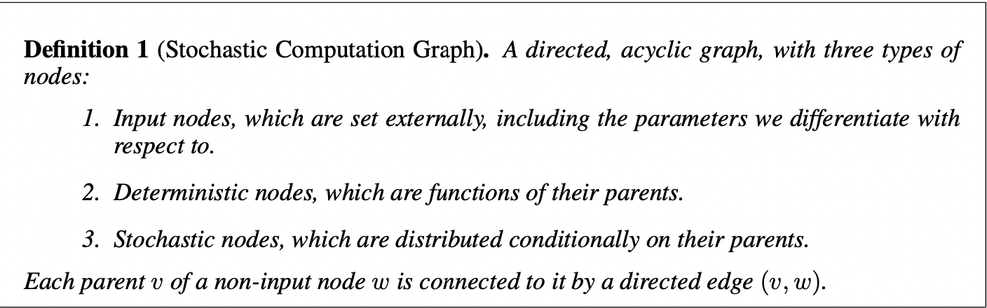
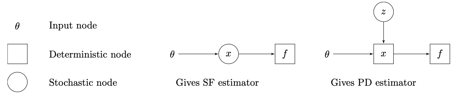
Where square denotes deterministic node, circle denotes stochastic node.
For simplification, \(E_Y [\cdot]\) denotes that \(Y\) are sampled from its distribution specified. P used for distribution, p for density function
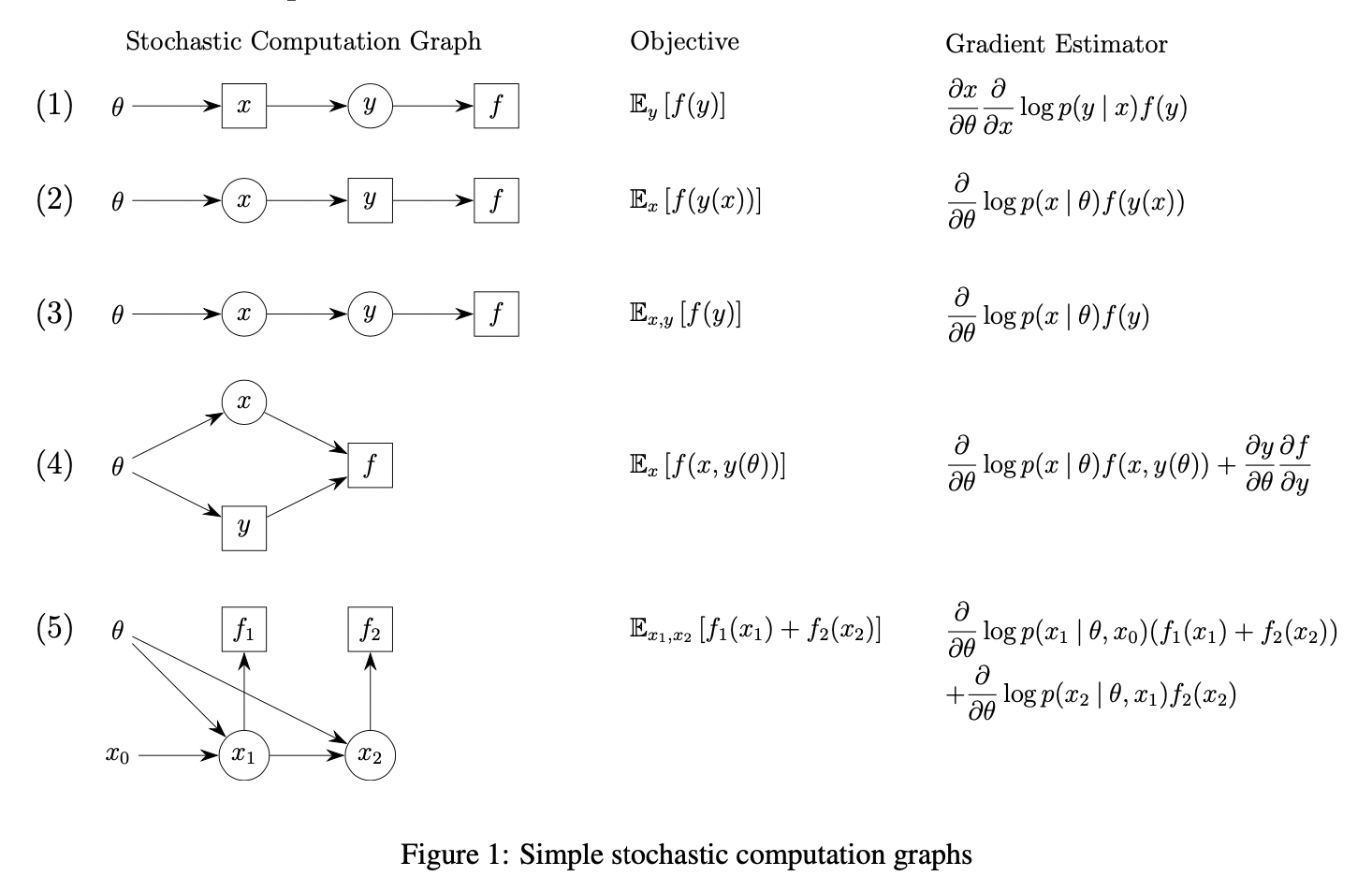
\(x(\theta), Y \sim P_Y(\cdot | x(\theta)), E_{Y \sim P_Y(\cdot | x(\theta))}[f(Y)]\) (the distribution depends on function of \(\theta\))
\[\frac{\partial }{\partial \theta} E_{Y \sim P_Y(\cdot | x(\theta))}[f(Y)] = \int_y p(y | x(\theta)) \frac{\partial log p(y | x(\theta))}{\partial \theta}\frac{\partial x(\theta)}{\partial \theta} dy = E_Y[\frac{\partial log p(Y | x(\theta))}{\partial \theta}\frac{\partial x(\theta)}{\partial \theta}]\]
\(X \sim P_X(\cdot | \theta), Y(X), f(Y(X))\) (the distribution depends on \(\theta\))
\[\frac{\partial }{\partial \theta} E_X[f(Y(X))] = \int_x p(x | \theta) \frac{\partial }{\partial \theta} log p(x | \theta) f(Y(x)) dx = E_X [log p(X | \theta) f(Y(X))]\]
\(X \sim P_X(\cdot | \theta), Y \sim P_Y(\cdot | X), f(Y)\) (the distribution depends on \(\theta\))
\[\frac{\partial }{\partial \theta} E_{X, Y}[f(Y)] = \int_y \int_x p(x | \theta) p(y | x) f(y)\frac{\partial }{\partial \theta} log p(x | \theta) dx dy = E_{X, Y} [log p(X | \theta) f(Y)]\]
\(X \sim P_X(\cdot | \theta), y(\theta), f(X, y(\theta))\) (the distribution depends on \(\theta\) and the function \(f\) depends on \(\theta\))
\[\frac{\partial }{\partial \theta} E_{X}[f(X, y(\theta))] = \int_x p(x | \theta) \frac{\partial }{\partial \theta} log p(x | \theta) f(x, y(\theta)) + p(x | \theta) \frac{\partial f(x, y(\theta))}{\partial y(\theta)} \frac{\partial y(\theta)}{\partial \theta} dx = E_X [\frac{\partial }{\partial \theta} log p(X | \theta) f(X, y(\theta)) + \frac{\partial f(X, y(\theta))}{\partial y(\theta)} \frac{\partial y(\theta)}{\partial \theta}]\]
\(X_1 \sim P_{X_1}(\cdot | \theta, x_0), X_2 \sim P_{X_2}(\cdot | \theta, X_1), f_1 (X_1), f_2 (X_2)\) (Notice that \(X_2\) has no effect on the distribution of \(X_1\), this resembles a parameterized Markov reward process, and it illustrates that we’ll obtain score function terms of the form grad log-probability times future costs.)
\[\begin{aligned} \frac{\partial }{\partial \theta} E_{X_1, X_2}[f_1(X_1), f_2(X_2)] &= \frac{\partial }{\partial \theta} (E_{X_1} [f_1(X_1)] + E_{X_1, X_2} [f_2(X_2)]) \\ &= \int_{x_1} p(x_1 | \theta) \frac{\partial }{\partial \theta} log p(x_1 | \theta) f_1 (x_1) dx_1 + \int_{x_1} \int_{x_2} p(x_2 | \theta)p(x_1 | \theta) \frac{\partial }{\partial \theta} log p(x_2 | \theta) f_2 (x_2) + p(x_2 | \theta)p(x_1 | \theta) \frac{\partial }{\partial \theta} log p(x_1 | \theta) f_2 (x_2)dx_2 dx_1 \\ &= E_{X_1, X_2}[\frac{\partial }{\partial \theta} log p(X_1 | \theta) (f(X_1) + f(X_2)) + \frac{\partial }{\partial \theta} log p(X_2 | \theta) f(X_2)] \end{aligned}\]
Main Results
Gradient Estimation
Notations
The set of cost nodes \(C\) are
scalar-valuedanddeterministic(There is no loss of generality in assuming that the costs are deterministic, if a cost is stochastic, we can simply append a deterministic node that applies hte identity function to it).The relation \(v \prec w\) means that \(\exists\) a sequence of nodes \(a_1, ...., a_K\) with \(K \leq 0\) such that \((v, a_1), ...., (a_K, w)\) are edges in the graph (Basicly, there exists a
pathfrom \(v\) to \(w\))The relation \(v \prec^D w\) means that all sequence of nodes \(a_1, ...., a_K\) are deterministic (Also, if (\(v\), \(w\)) is an edge in the graph, then \(v \prec^D w\))
\(\hat{Q_v} \triangleq \sum_{ c \succ v, c \in C} \hat{c}\), this is the sum of costs influenced by node \(v\).
All
hatsare denoted as sample realizations of random variables and are regarded asconstant.\(\text{DEPS}_{v} \triangleq \{ w \in \Theta \bigcup S \; | \; w \prec^D v \}\):
- If \(v \in S\), then we can write \(p(v \; | \; \text{DEPS}_{v})\)
- If \(v \in D\), then we can write \(v\) as function of \(\text{DEPS}_{v}\): \(v(\text{DEPS}_{v})\)
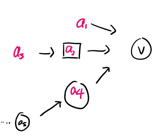
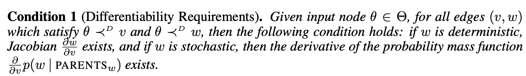
In this case,
- If \(v\) is deterministic, then it is a function that depends on \(v(a_1, a_2(a_3), a_4)\) but not \(a_5\).
- If \(v\) is stochastic, then it's probability distribution depends on \(P( \cdot |a_1, a_2(a_3), a_4)\) but not \(a_5\)
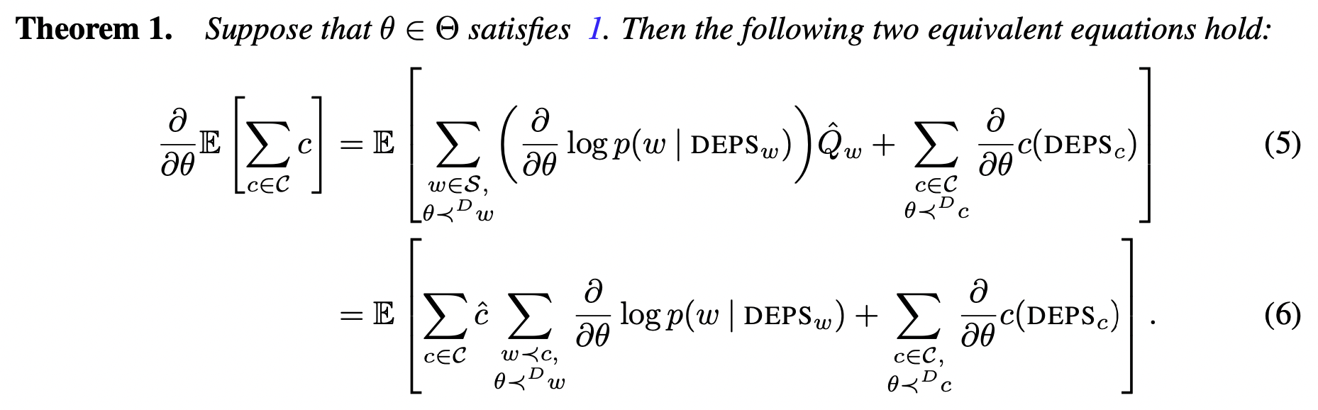
Assume that:
Theorem 1
Proof
Consider only \(v \in S\), \(E_{v \in S, v \prec c}[c]\):
\[\begin{aligned} E_{v \in S, v \prec c}[c] &= \int_{v} p(v_1 \; | \; \text{DEPS}_{v_1}) p(v_2 \; | \; \text{DEPS}_{v_2}) ... p(v_k \; | \; \text{DEPS}_{v_k})c(\text{DEPS}_{c})dv\\ &= \int_{v} c(\text{DEPS}_{c}) \prod_{v} p(v \; | \; \text{DEPS}_{v})dv \end{aligned}\]Here, \(c\) is deterministic node, by definition it is a function of its dependencies. \(v = \{v_1, ..., v_k\}\) is a set of stochastic nodes, so all of them have probability density or mass functions that depends on their dependencies.
Then the derivative \(\frac{\partial}{\partial \theta}E_{v \in S, v \prec c}[c]\) w.r.t \(\theta\) is:
\[\begin{aligned} \frac{\partial}{\partial \theta} E_{v \in S, v \prec c}[c] &= \frac{\partial}{\partial \theta} \int_{v} c(\text{DEPS}_{c}) \prod_{v} p(v \; | \; \text{DEPS}_{v})dv\\ &= \int_{v} \frac{\partial c(\text{DEPS}_{c})}{\partial \theta} \prod_{v} p(v \; | \; \text{DEPS}_{v})dv + \int_{v} c(\text{DEPS}_{c}) \frac{\partial \prod_{v} p(v \; | \; \text{DEPS}_{v})}{\partial \theta}dv\\ &= \int_{v} \frac{\partial c(\text{DEPS}_{c})}{\partial \theta} \prod_{v} p(v \; | \; \text{DEPS}_{v})dv + \int_{v} c(\text{DEPS}_{c}) \prod_{v} p(v \; | \; \text{DEPS}_{v}) \sum_{w \in S, w \prec c} \frac{\frac{\partial}{\partial \theta} p(w \; | \; \text{DEPS}_{w})}{p(w \; | \; \text{DEPS}_{w})}dv\\ &= \int_{v} \frac{\partial c(\text{DEPS}_{c})}{\partial \theta} \prod_{v} p(v \; | \; \text{DEPS}_{v})dv + \int_{v} c(\text{DEPS}_{c}) \prod_{v} p(v \; | \; \text{DEPS}_{v}) \sum_{w \in S, w \prec c} \frac{\partial}{\partial \theta} \log (p(w \; | \; \text{DEPS}_{w}))dv\\ &= E_{v \in S, v \prec c} [\frac{\partial c(\text{DEPS}_{c})}{\partial \theta} + \hat{c} \sum_{w \in S, w \prec c} \frac{\partial}{\partial \theta} \log (p(w \; | \; \text{DEPS}_{w}))] \\ \end{aligned}\]Recall that if \(\theta \prec^D w\) then \(\theta \in \text{DEPS}_{w}\). Notice here, terms in the sum \(\sum_{w \in S, w \prec c} \frac{\partial}{\partial \theta} \log (p(w \; | \; \text{DEPS}_{w}))\) that do not depend on \(\theta\) will have 0 gradients, thus, we can rewrite:
\[\sum_{w \in S, w \prec c} \frac{\partial}{\partial \theta} \log (p(w \; | \; \text{DEPS}_{w})) = \sum_{w \in S, w \prec c, \theta \prec^D w} \frac{\partial}{\partial \theta} \log (p(w \; | \; \text{DEPS}_{w}))\]
At the same time, we can substitute \(\hat{c}\) for \(c\), which does not affect the expectation.
More generally, we can have \(v\) being either stochastic or deterministic:
\[v \prec c\]
Then,
\[\begin{aligned} \frac{\partial}{\partial \theta}E_{v \prec C}[\sum_{c \in c} c] &= \frac{\partial}{\partial \theta} \sum_{c \in C} E_{v \prec c}[c]\\ &= \sum_{c \in C} E_{v \prec c} [\frac{\partial c(\text{DEPS}_{c})}{\partial \theta} + \hat{c}\sum_{w \prec c, \theta \prec^D w} \frac{\partial}{\partial \theta} \log (p(w \; | \; \text{DEPS}_{w}))]\\ &= E_{v \in S, v \prec c} [ \sum_{c \in C} \frac{\partial c(\text{DEPS}_{c})}{\partial \theta} + \sum_{c \in C}\hat{c} \sum_{w \prec c, \theta \prec^D w} (\frac{\partial}{\partial \theta} \log (p(w \; | \; \text{DEPS}_{w})))]\\ &= E_{v \in S, v \prec c} [ \sum_{c \in C} \frac{\partial c(\text{DEPS}_{c})}{\partial \theta} + \sum_{w \prec S, \theta \prec^D w} (\frac{\partial}{\partial \theta} \log (p(w \; | \; \text{DEPS}_{w}))) \hat{Q}_{w}]\\ \end{aligned}\]The estimated expressions above have two terms:
- The first term is due to the influence of \(\theta\) on the probability distributions.
- The second term is due to the influence of \(\theta\) on the cost variables through a chain of differentiable functions.
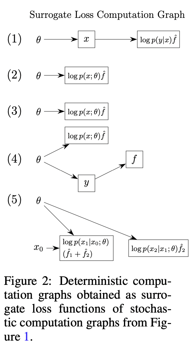
Surrogate Loss Functions
The next corollary lets us write down a surrogate objective \(L\), which is a function of the inputs that we can differentiate to obtain an unbiased gradient estimator.
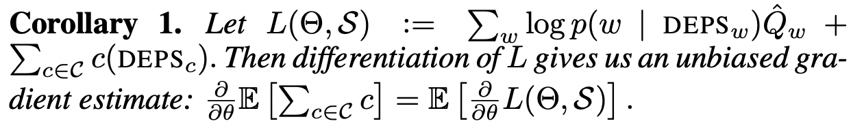
We now convert a stochastic computation graph to a deterministic computation graph, and we can apply automatic differentiation.
Algorithm