Policy Gradient (2)
Policy Search Methods (Policy Gradient)
All \(\nabla\) refer to \(\nabla_{\theta}\) for simplicity.
From introduction blog, our goal:
\[\underset{\pi_{\theta}}{\operatorname{maximize}} J_\rho(\pi_\theta) = \underset{\theta}{\operatorname{maximize}} J_\rho(\pi_\theta)\]
By taking the gradient w.r.t \(\theta\), we have:
\[\begin{aligned} \nabla J_\rho(\pi_\theta) &= \nabla E_{X_1 \sim \rho} [V^{\pi_\theta} (X_1)]\\ &= \nabla \int_{x_1}\int_{a} [r(x_1, a) \pi_{\theta} (a | x_1) da dx_1 + \int_{x^{\prime}} P(x^{\prime} | x_1, a) \pi_{\theta}(a | x_1) V^{\pi_\theta}(x^{\prime})dx^{\prime} da dx_1]\\ &= \nabla \int_{a} \int_{x_1} \int_{x^{\prime}} \pi_{\theta}(a | x_1) [r(x_1, a) + P(x^{\prime} | x_1, a) V^{\pi_\theta}(x^{\prime})]dx^{\prime} da dx_1 \\ &= \int_{x_1} \int_{a} \int_{x^{\prime}} \nabla [\pi_{\theta}(a | x_1) (r(x_1, a) + P(x^{\prime} | x_1, a) V^{\pi_\theta}(x^{\prime}))]dx^{\prime} da dx_1 \\ \end{aligned}\]We can swap integral and derivative as long as \(V^{\pi_{\theta}}\) is a continuous function of \(\theta\), the estimator of this expectation is called pathwise derivative estimator or stochastic backpropagation estimator (more details in Stochastic Graph).
This \(\nabla J_\rho(\pi_\theta)\) is called the Policy Gradient. In ideal case, if we know the policy gradient (i.e if we know the environment dynamics \(P, R\)), we can use gradient ascent to update the parameters \(\theta\).
The question is, how can we approximate this gradient in reality using samples?
Immediate Reward Problem (Easy Case)
First, let's consider an immediate reward problem:
In this setting, our \(J_\rho(\pi_\theta)\) is:
\[\begin{aligned} J_\rho(\pi_\theta) &= \int_{x_1} V^{\pi_\theta} \rho(x_1) dx_1 \\ &= \int_{x_1} \int_{a} r(x_1, a) \pi_{\theta}(a | x_1) \rho(x_1) da dx_1 \\ \end{aligned}\]The value function \(V^{\pi_\theta}\) in this setting is the same as \(r^{\pi_{\theta}}\), and the action space is continuous.
Then, the policy gradient \(\nabla J_\rho(\pi_\theta)\) can be written as:
\[\nabla J_\rho(\pi_\theta) = \int_{x_1} \int_{a} r(x_1, a) \rho(x_1) \nabla \pi_{\theta}(a | x_1) da dx_1\]
How can we compute \(\nabla J_\rho(\pi_\theta)\) ?
Recall that, \(\frac{\partial log (\theta)}{ \partial \theta} = \frac{1}{\theta}\):
\[\begin{aligned} \nabla J_\rho(\pi_\theta) &= \int_{x_1} \int_{a} r(x_1, a) \rho(x_1) \nabla \pi_{\theta}(a | x_1) da dx_1\\ &= \int_{x_1} \int_{a} r(x_1, a) \rho(x_1) \pi_{\theta}(a | x_1) \frac{\nabla \pi_{\theta}(a | x_1)}{\pi_{\theta}(a | x_1)} da dx_1\\ &= \int_{x_1} \int_{a} \rho(x_1) \pi_{\theta}(a | x_1) r(x_1, a) \nabla log (\pi_{\theta}(a | x_1)) da dx_1\\ &= E_{X_1 \sim \rho, A \sim \pi_{\theta}(\cdot | X_1)} [r(X_1, A) \nabla log (\pi_{\theta}(A | X_1))] \end{aligned}\]Then, we can draw samples from this expectation:
\[r(X_1, A) \nabla log (\pi_{\theta}(A | X_1))\]
These samples are called REINFORCE or Score function estimators. These samples are unbiased samples of the policy gradient \(\nabla J_\rho(\pi_\theta)\). We can use these unbiased but noisy samples to update parameters. This makes it Stochastic Gradient Ascent.
Baseline
We know that above sample is unbiased sample of the policy gradient, but, how about its variance?
There are two source of variance:
- Variance that comes from sampling \(X_1 \sim \rho\) and use this sample to estimate the expectation.
- Variance that comes from sampling \(A \sim \pi_{\theta}(a | X_1)\) and use this sample to estimate the expectation.
Recall the total variance formula:
\[Var[Y] = E_X[Var[Y | X]] + Var_X[E[Y | X]]\]
One can show that the variance for \(i\)th dimension of \(\nabla J_\rho(\pi_\theta)\):
\[Var[r(X_1, A) \frac{\partial}{\partial \theta_i} log (\pi_{\theta}(A | X_1))] = E_{X_1} [Var_{A}[r(X_1, A) \frac{\partial}{\partial \theta_i} log (\pi_{\theta}(A | X_1)) | X_1]] + Var_{X_1} [E_A[r(X_1, A) \frac{\partial}{\partial \theta_i} log (\pi_{\theta}(A | X_1)) | X_1]]\]
To see this more clearly, let's define:
\[g(x; \theta) = E_{A \sim \pi_{\theta}(\cdot | x)} [r(x, A) \nabla log (\pi_{\theta}(A | x))]\]
This function \(g: X \times \Theta \rightarrow \mathbb{R}^{p}\) is the policy gradient at a particular starting state \(x\), and it is a \(p\)-dimensional vector (Assuming \(\theta\) is \(p\)-dimensional). Then we have:
\[Var[r(X_1, A) \frac{\partial}{\partial \theta_i} log (\pi_{\theta}(A | X_1))] = E_{X_1} [Var_{A}[r(X_1, A) \frac{\partial}{\partial \theta_i} log (\pi_{\theta}(A | X_1)) | X_1]] + Var_{X_1} [g_i(X_1; \theta)]\]
These two sources of variance make our estimate of the gradient inaccurate. We can reduce them using a baseline.
Consider the variance of estimating \(g(x; \theta)\) using a single sample \(r(x, A) \nabla log (\pi_{\theta}(A | x))\) with \(A \sim \pi_\theta(\cdot | x)\). For each dimension \(i\), we have:
\[\begin{aligned} E_{A}[ (r(x, A) - b(x)) \frac{\partial}{\partial \theta_i}log (\pi_{\theta}(A | x)) \; |\; x] &= \int_a (r(x, a) - b(x)) \pi_{\theta}(a | x) \frac{\partial}{\partial \theta_i} log (\pi_{\theta}(a | x)) da\\ &= \int_a r(x, a) \frac{\partial}{\partial \theta_i} \pi_{\theta}(a | x) da - b(x) \int_a \frac{\partial}{\partial \theta_i} \pi_{\theta}(a | x) da\\ &= \int_a r(x, a) \frac{\partial}{\partial \theta_i} \pi_{\theta}(a | x) da - b(x) \frac{\partial}{\partial \theta_i} \underbrace{\int_a \pi_{\theta}(a | x) da}_{1} \\ &= \int_a r(x, a) \frac{\partial}{\partial \theta_i} \pi_{\theta}(a | x) da - b(x) \frac{\partial}{\partial \theta_i} (1)\\ &= \int_a r(x, a) \frac{\partial}{\partial \theta_i} \pi_{\theta}(a | x) da\\ &= E_{A}[ (r(x, A) - b(x)) \frac{\partial}{\partial \theta_i}log (\pi_{\theta}(A | x))\; |\; x] \end{aligned}\]This shows that, if we add a state dependent function \(b(x)\) to \(r(x, a)\), the expectation won't change. But, this may change the variance! We can formulate this idea to be an optimization problem and find a function \(b: X \rightarrow \mathbb{R}^{p}\) such that for all \(x \in X\) (for each \(b_i\)):
\[\min_{b_i} \sum^{p}_{i=1} Var[(r(x, A) + b_i (x)) \frac{\partial}{\partial \theta_i}log (\pi_{\theta}(A | x)) \; |\; x]\]
by solving this optimization problem, we have:
\[b_i (x) = \frac{-E_A[r(x, A) (\frac{\partial}{\partial \theta_i}log (\pi_{\theta}(A | x)))^2 \; |\; x]}{E_A [(\frac{\partial}{\partial \theta_i}log (\pi_{\theta}(A | x)))^2 | x]}\]
We can also choose single scalar function \(b: X \rightarrow \mathbb{R}\) instead:
\[b (x) = \frac{-E_A[r(x, A) \|\frac{\partial}{\partial \theta_i}log (\pi_{\theta}(A | x))\|^2_2 \; |\; x]}{E_A [\|\frac{\partial}{\partial \theta_i}log (\pi_{\theta}(A | x))\|^2_2 | x]}\]
Policy Gradient (General Case)
Recall that:
\[P^{\pi} (\cdot | y)= \int_{x \in X} \int_a P(x | y, a) \pi(a | y) da dx\]
Average Reward Setting
The difference with the immediate reward case, where we only need initial distribution \(\rho\), in average reward case, we depend on the environment transition distribution \(P^{\pi_{\theta}}\) too. As we update \(\theta\), we obtain a different policy \(\pi_{\theta}\), that is, we have a different dynamics transition distribution \(P^{\pi_{\theta}}\).
Recall that in average reward setting, the quality of a policy is measured as the long term expected reward or average rate reward or simply average reward following \(\pi_\theta\) independent of starting state (\(x_1\) in the expectation is used to emphasize that the Expected reward is \(t\) step):
Where \(\rho^{\pi_{\theta}} (x) = \lim_{n \rightarrow \infty}\frac{1}{n} \sum^{n}_{t=1} P^{\pi_{\theta}} (X_t = x | x_1; t) = \lim_{t \rightarrow \infty} P^{\pi_{\theta}} (X_t = x | x_1; t)\).
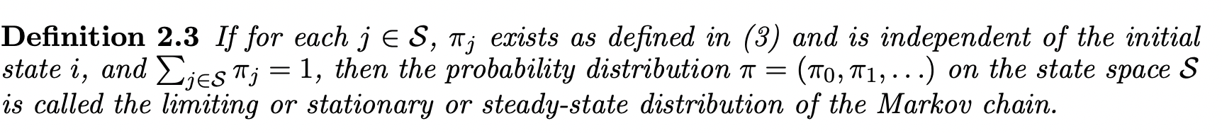
Stationary Distribution
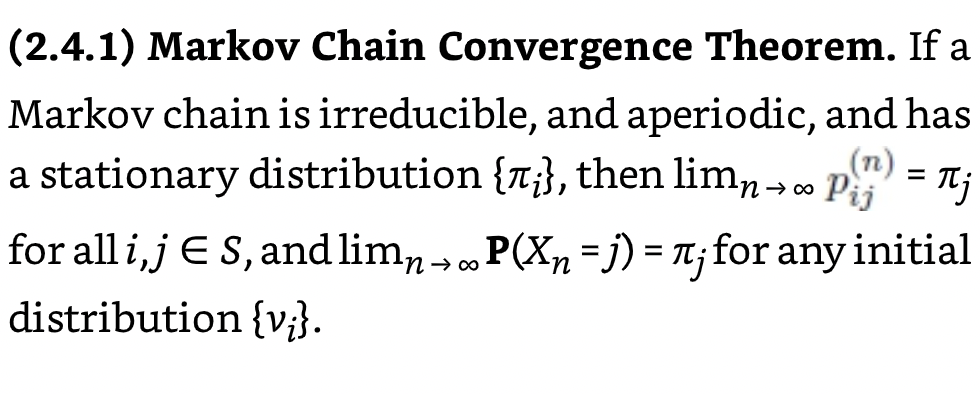
\(\rho^{\pi_{\theta}}\) above is the stationary distribution under \(\pi_\theta\) which is assumed to exist (when the markov chain is ergodic) and independent of starting state (\(x_1\) here is used to emphasize that this is \(t\) step transition probability).
In general, let \(\sum^{N}_{n=1}I\{X_n = j | X_0=i \}\) be the number of visits to state \(j\) in \(N\) steps starting from \(i\). Then the expected visits to state \(j\) is:
\[E[\sum^{N}_{n=1}I\{X_n = j | X_0=i\}] = \sum^{N}_{n=1} E[I\{X_n = j\} | X_0=i] = \sum^{N}_{n=1} P(X_n=j | X_0=i)\]
The expected proportion of visits is then:
\[\frac{\sum^{N}_{n=1} P(X_n=j | X_0=i)}{N}\]
The stationary distribution can be interpreted as the long run expected proportion of time that the chain spends for each state over the state space, so it is defined as \(\pi = (\pi_0, \pi_1, ...)\) over the state space \(X\):
So \(\rho^{\pi_{\theta}} (\cdot)\) is the special distribution in which if you select actions according to \(\pi_\theta\), you end up in the same distribution:
\[\int_{x} \rho^{\pi_{\theta}} (x) \int_a \pi_{\theta}(a | x) \int_{x^{\prime}} P(x^{\prime} | x, a) dx^{\prime} da dx = \rho^{\pi_{\theta}} (x^{\prime})\]
We can easily sample states from this distribution by following \(\pi_{\theta}\).
Discounted Setting
In discounted setting, the objective is defined as long term discounted return starting from initial state distribution \(X_1 \sim \rho\) following \(\pi_{\theta}\):
\[J_{\rho} (\pi_\theta) = E_{X_1 \sim \rho} [V^{\pi_{\theta}} (X_1)]\]
Recall that \(P^{\pi_{\theta}} (\cdot | x; k) = P^{\pi_{\theta}} (\cdot | x)^k\) is the \(k\) step transition distribution:
\[\sum^{\infty}_{k=0} \gamma^k P^{\pi_{\theta}} (X_{k + 1}=x | x_{1}) = P^{\pi_{\theta}}(X_{1} = x | x_{1}) + \gamma P^{\pi_{\theta}}(X_{2} = x | x_{1}) + ...\]
By taking the expected value over initial state we have:
\[\begin{aligned} E_{x_1} [\sum^{\infty}_{k=0} \gamma^k P^{\pi_{\theta}} (X_{k + 1}=x | x_{1})] &= E_{x_1} [P^{\pi_{\theta}}(X_{1} = x | x_{1})] + \gamma E_{x_1} [P^{\pi_{\theta}}(X_{2} = x | x_{1})] \; + ...\\ &= \rho(x) + \gamma \sum_{x_1} P^{\pi_{\theta}}(X_{2} = x | x_{1}) \rho(x_1) \; + ...\\ &= \rho(x) + \gamma P^{\pi_{\theta}}(X_{2} = x) \; + ...\\ &= Pr(X_1 = x) + \gamma Pr(X_{2} = x) \; + ... \\ \end{aligned}\]This is the expected number of time steps spend in state \(x\) discounted by \(\gamma^k\) given we start at state \(X_1 \sim \rho\).
Let's now define the discounted future state distribution (similar to stationary distribution but with discount and depend on initial state)starting from state \(x_1 \in X\) following \(\pi_{\theta}\):
\[\rho^{\pi}_{\gamma} (\cdot | x_1) \triangleq (1 - \gamma) \sum^{\infty}_{k=0} \gamma^k P^{\pi_{\theta}} (\cdot | x_1; k)\]
Where , and \(1 - \gamma\) is the normalization term. We can easily verify that this is a valid distribution. One interpretation of this distribution is that the agent starts at \(x_1\) and at each time step \(t\) terminate with probability \(1 - \gamma\). This accounts for the discounted factor inside the average counts. That is, we can sample from the state stationary distribution and terminate at each step with probability \(1 - \gamma\). Or instead, we could weight each samples by \(\gamma^k\) to account for the termination.
We can also define the discounted future-state distribution of starting from \(\rho\) and following \(\pi\) as:
\[\rho^{\pi}_{\gamma} (\cdot) = \int_{x_1} \rho^{\pi}_{\gamma} (\cdot | x_1) \rho (x_1) dx_1\]
\[\rho^{\pi}_{\gamma} (x) = (1 - \gamma) E_{x_1} [\sum^{\infty}_{k=0} \gamma^k P^{\pi} (X_{k + 1}=x | x_{1})] = (1 - \gamma)(Pr(X_1 = x) + \gamma Pr(X_{2} = x) \; + ...) \]
Expected Reward and Discounted Return
We can see the connection between expected reward and discounted return:
\[\begin{aligned} V^{\pi} (x) &= E^{\pi}[\sum^{\infty}_{t = 1} \gamma^{t - 1} R_{t} \; |\; X_1 = x]\\ &= \sum^{\infty}_{t = 1} \gamma^{t - 1} E^{\pi}[R_{t} \; |\; X_1 = x]\\ &= \sum^{\infty}_{t = 1} \gamma^{t - 1} \int_{x^{\prime}, a} P^{\pi}(X_t=x^{\prime} | x; t) \pi(a | x^{\prime})R(x^{\prime}, a)da dx^{\prime}\\ &= \frac{1}{1 - \gamma} \int_{x^{\prime}, a} \rho^{\pi}_{\gamma} ( x^{\prime}| x) \pi(a | x^{\prime}) R(x^{\prime}, a) dadx^{\prime}\\ &= \frac{1}{1 - \gamma}E_{X^{\prime} \sim \rho^{\pi}_{\gamma} (\cdot | x), A \sim \pi(\cdot | X^{\prime})} [R(X^{\prime}, A)]\\ \end{aligned}\]We can interchange summation and infinity sum because the sum is finite. Here \(R(\cdot)\) represents the realization of random variable \(R\). This tells us that the value function at a state \(x\) is the expected reward when \(X^{\prime}\) is distributed according to \(\rho^{\pi}_{\gamma} (\cdot | x)\) and following \(\pi\).
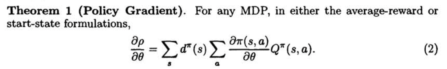
Policy Gradient Theorem
Proof: Average Reward Setting
In average reward setting, \(d^{\pi} (x) = \rho^{\pi_{\theta}} (x),\; \; \rho = J (\pi_\theta)\) and \(Q^{\pi} (x, a)\) is defined as:
\[Q^{\pi} (x, a) = r(x, a) - J(\pi_\theta) + \int_{x^{\prime}} P(x^{\prime} | x, a) V^{\pi_{\theta}} (x^{\prime}) dx^{\prime}\]
Recall that,
\[\begin{aligned} \nabla V^{\pi_{\theta}} (x) &= \int_{a} \pi_{\theta}(a | x) Q^{\pi_{\theta}} (x, a) da \;\;\;\;\;\;\;\;\;\;\;\;\;\;\; \forall x \in X\\ &= \int_{a} \nabla \pi_{\theta}(a | x) Q^{\pi_{\theta}} (x, a) da + \int_a \pi_{\theta}(a | x) \nabla Q^{\pi_{\theta}} (x, a) da\\ &= \int_{a} \nabla \pi_{\theta}(a | x) Q^{\pi_{\theta}} (x, a) da + \int_a \pi_{\theta}(a | x) \nabla (r(x, a) - J(\pi_\theta) + \int_{x^{\prime}} P(x^{\prime} | x, a) V^{\pi_{\theta}} (x^{\prime})dx^{\prime}) da\\ &= \int_{a} \nabla \pi_{\theta}(a | x) Q^{\pi_{\theta}} (x, a) da + \int_a \pi_{\theta}(a | x) (- \nabla J(\pi_\theta) + \int_{x^{\prime}} P(x^{\prime} | x, a) \nabla V^{\pi_{\theta}} (x^{\prime})dx^{\prime}) da\\ \end{aligned}\]That is:
\[\nabla J(\pi_\theta) \underbrace{\int_a \pi_{\theta}(a | x) da}_{1} = \int_{a} \nabla \pi_{\theta}(a | x) Q^{\pi_{\theta}} (x, a) da + \int_a \pi_{\theta}(a | x) \int_{x^{\prime}} P(x^{\prime} | x, a) \nabla V^{\pi_{\theta}} (x^{\prime})dx^{\prime} da - \nabla V^{\pi_{\theta}} (x)\]
Weighting both sides by (taking expectation) \(\rho^{\pi_{\theta}} (x)\) and remember the property of stationary distribution \(\int_{x} \rho^{\pi_{\theta}} (x) \int_a \pi_{\theta}(a | x) \int_{x^{\prime}} P(x^{\prime} | x, a) dx^{\prime} da dx = \rho^{\pi_{\theta}} (x^{\prime})\):
\[\begin{aligned} \underbrace{\int_{x} \rho^{\pi_{\theta}} (x) dx}_{1} \nabla J(\pi_\theta) &= \int_{x} \rho^{\pi_{\theta}} (x) \int_{a} \nabla \pi_{\theta}(a | x) Q^{\pi_{\theta}} (x, a) da dx + \int_{x} \rho^{\pi_{\theta}} (x) \int_a \pi_{\theta}(a | x) \int_{x^{\prime}} P(x^{\prime} | x, a) \nabla V^{\pi_{\theta}} (x^{\prime})dx^{\prime} da dx- \int_{x} \rho^{\pi_{\theta}} (x) \nabla V^{\pi_{\theta}} (x) dx \\ \nabla J(\pi_\theta) &= \int_{x} \rho^{\pi_{\theta}} (x) \int_{a} \nabla \pi_{\theta}(a | x) Q^{\pi_{\theta}} (x, a) da dx + \int_{x} \rho^{\pi_{\theta}} (x) \int_a \pi_{\theta}(a | x) \int_{x^{\prime}} P(x^{\prime} | x, a) \nabla V^{\pi_{\theta}} (x^{\prime})dx^{\prime} da dx- \int_{x} \rho^{\pi_{\theta}} (x) \nabla V^{\pi_{\theta}} (x) dx \\ &= \int_{x} \rho^{\pi_{\theta}} (x) \int_{a} \nabla \pi_{\theta}(a | x) Q^{\pi_{\theta}} (x, a) da dx + \int_{x^{\prime}} \rho^{\pi_{\theta}} (x^{\prime}) \nabla V^{\pi_{\theta}} (x^{\prime})dx- \int_{x} \rho^{\pi_{\theta}} (x) \nabla V^{\pi_{\theta}} (x) dx \\ &= \int_{x} \rho^{\pi_{\theta}} (x) \int_{a} \nabla \pi_{\theta}(a | x) Q^{\pi_{\theta}} (x, a) da dx \\ \end{aligned}\]Proof: Discounted Return Setting
In discounted return setting, \(d^{\pi} (x) = \rho^{\pi_{\theta}} (x),\; \; \rho = J_{\rho} (\pi_\theta)\).
Recall that,
\[\begin{aligned} \nabla V^{\pi_{\theta}} (x) &= \int_{a} \pi_{\theta}(a | x) Q^{\pi_{\theta}} (x, a) da \;\;\;\;\;\;\;\;\;\;\;\;\;\;\; \forall x \in X\\ &= \int_{a} \nabla \pi_{\theta}(a | x) Q^{\pi_{\theta}} (x, a) da + \int_a \pi_{\theta}(a | x) \nabla Q^{\pi_{\theta}} (x, a) da\\ &= \int_{a} \nabla \pi_{\theta}(a | x) Q^{\pi_{\theta}} (x, a) da + \int_a \pi_{\theta}(a | x) \nabla (r(x, a) + \int_{x^{\prime}} P(x^{\prime} | x, a) \gamma V^{\pi_{\theta}} (x^{\prime})dx^{\prime}) da\\ &= \int_{a} \nabla \pi_{\theta}(a | x) Q^{\pi_{\theta}} (x, a) da + \int_a \pi_{\theta}(a | x) \int_{x^{\prime}} P(x^{\prime} | x, a) \gamma \nabla V^{\pi_{\theta}} (x^{\prime})dx^{\prime} da\\ &= \int_{a} \nabla \pi_{\theta}(a | x) Q^{\pi_{\theta}} (x, a) da + \int_a \pi_{\theta}(a | x) \int_{x^{\prime}} P(x^{\prime} | x, a) \gamma \nabla V^{\pi_{\theta}} (x^{\prime})dx^{\prime} da\\ &= \int_{a} \nabla \pi_{\theta}(a | x) Q^{\pi_{\theta}} (x, a) da + \int_{x^{\prime}} P^{\pi_{\theta}}(x^{\prime} | x) \gamma \nabla V^{\pi_{\theta}} (x^{\prime})dx^{\prime}\\ \end{aligned}\]Now we expand \(V^{\pi_{\theta}} (x^{\prime})\) likewise, we will end up with the recursive relation:
\[\nabla V^{\pi_{\theta}} (x) = \int_{x^{\prime}} \sum^{\infty}_{k = 0}\gamma^k P^{\pi_\theta} (x^{\prime} | x; k) \int_{a^{\prime}} \nabla \pi_{\theta}(a^{\prime} | x^{\prime}) Q^{\pi_{\theta}} (x^{\prime}, a^{\prime}) da^{\prime} dx^{\prime}\]
Then, we can make this an expectation by adding normalization term:
\[\begin{aligned} \nabla V^{\pi_{\theta}} (x) &= \frac{1}{1 - \gamma}\int_{x^{\prime}} (1 - \gamma) \sum^{\infty}_{k = 0}\gamma^k P^{\pi_\theta} (x^{\prime} | x; k) \int_{a^{\prime}} \nabla \pi_{\theta}(a^{\prime} | x^{\prime}) Q^{\pi_{\theta}} (x^{\prime}, a^{\prime}) da^{\prime} dx^{\prime}\\ &= \frac{1}{1 - \gamma} \int_{x^{\prime}} \rho^{\pi_{\theta}} (x^{\prime} | x) \int_{a^{\prime}} \nabla \pi_{\theta}(a^{\prime} | x^{\prime}) Q^{\pi_{\theta}} (x^{\prime}, a^{\prime}) da^{\prime} dx^{\prime}\\ \end{aligned}\]Then \(\nabla J_{\rho} (\pi_\theta) = E_{X \sim \rho}[\nabla V^{\pi_{\theta}} (X)]\) can be expressed as:
\[\begin{aligned} \nabla J_{\rho} (\pi_\theta) &= \frac{1}{1 - \gamma} \int_{x_1} \int_{x^{\prime}} \rho(x_1) \rho^{\pi_{\theta}} (x^{\prime} | x_1) \int_{a^{\prime}} \nabla \pi_{\theta}(a^{\prime} | x^{\prime}) Q^{\pi_{\theta}} (x^{\prime}, a^{\prime}) da^{\prime} dx^{\prime} dx_1\\ &= \frac{1}{1 - \gamma} \int_{x^{\prime}} \rho^{\pi_{\theta}} (x^{\prime}) \int_{a^{\prime}} \nabla \pi_{\theta}(a^{\prime} | x^{\prime}) Q^{\pi_{\theta}} (x^{\prime}, a^{\prime}) da^{\prime} dx^{\prime}\\ \end{aligned}\]Policy Gradients as Expectations
Recall that, the score function estimator :
\[\frac{\partial}{\partial \theta} E_{X \sim p(\cdot ; \theta)}[f(X)] = \int_x \frac{\frac{\partial}{\partial\theta} p(x; \theta)}{p(x; \theta)} p(x; \theta) f(x)dx = E_{X \sim p(\cdot ; \theta)}[f(X) \frac{\partial}{\partial\theta} \log p(X; \theta)]\]
Thus, the results above can be written as:
Average Reward Setting:
\[\begin{aligned} \nabla J(\pi_\theta) &= \int_{x} \rho^{\pi_{\theta}} (x) \int_{a} \nabla \pi_{\theta}(a | x) Q^{\pi_{\theta}} (x, a) da dx \\ &= E_{X \sim \rho^{\pi_{\theta}} (\cdot)} [ \int_{a} \frac{\pi_{\theta}(a | X)}{\pi_{\theta}(a | X)}\nabla \pi_{\theta}(a | X) Q^{\pi_{\theta}} (X, a) da]\\ &= E_{X \sim \rho^{\pi_{\theta}} (\cdot)} [ \int_{a} \frac{\nabla \pi_{\theta}(a | X)}{\pi_{\theta}(a | X)}\pi_{\theta}(a | X) Q^{\pi_{\theta}} (X, a) da]\\ &= E_{X \sim \rho^{\pi_{\theta}} (\cdot)} [ \int_{a} \pi_{\theta}(a | X) \nabla \log \pi_{\theta}(a | X) Q^{\pi_{\theta}} (X, a) da]\\ &= E_{X \sim \rho^{\pi_{\theta}} (\cdot), A \sim \pi_{\theta} (\cdot | X)} [\nabla \log \pi_{\theta}(A | X) Q^{\pi_{\theta}} (X, A)]\\ \end{aligned}\]Discounted Return Setting:
\[\nabla J_{\rho}(\pi_\theta) \propto E_{X \sim \rho^{\pi_{\theta}} (\cdot), A \sim \pi_{\theta} (\cdot | X)} [\nabla \log \pi_{\theta}(A | X) Q^{\pi_{\theta}} (X, A)]\]
Now we have nice expectation over state distribution or discounted future state distribution, we can use samples to estimate the gradient.
Sampling from Expectations
Average Reward Setting
In average reward setting or in episodic tasks when we have \(\gamma = 1\), sampling from the expectation is straight forward. We can directly sample trajectories following \(\pi_{\theta}\), then the states would be samples from the stationary state distribution and actions would be samples from the policy.
Discounted Return Setting
In discounted return setting, however, sampling is a little tricky.
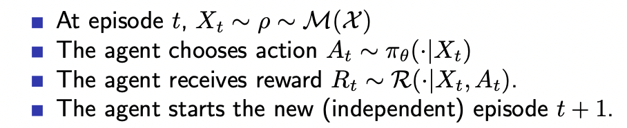
- The agent starts an episode from \(X_1 \sim \rho\) and follows \(\pi_\theta\)
- We get a sequence of states \(X_1, ...\)
However, these samples are from the stationary state distribution but not from the discounted future state distribution. In order to sample from the correct distribution, we either:
- Interpret \(\gamma\) as termination, terminate at each time step with probability \(1 - \gamma\).
- Add a weight \(\gamma^k\) which depends on the current time step to account for the discounting.
If we have sampled from the correct distribution and have an estimate for \(Q^{\pi_{\theta}} (X, A)\), we have an unbiased sample of the policy gradient:
\[\gamma^{k} \nabla \log \pi_{\theta}(A | X) Q^{\pi_{\theta}} (X, A)\]
We can now use these samples in an SG scheme to improve the policy.
Next: REINFORECE and A2C
Reference
Amir-massoud Farahmand. Introduction to Reinforcement Learning (Spring 2021) Lecture 6
Sham M. Kakade. On the sample complexity of reinforcement learning. 2003. https://homes.cs.washington.edu/~sham/papers/thesis/sham_thesis.pdf
Thomas, P.. (2014). Bias in Natural Actor-Critic Algorithms. Proceedings of the 31st International Conference on Machine Learning, in PMLR 32(1):441-448
Sutton, R. S., McAllester, D. A., Singh, S. P., and Man- sour, Y. (1999). Policy gradient methods for reinforce- ment learning with function approximation. In Neural Information Processing Systems 12, pages 1057–1063.
Sutton & Barto's "Reinforcement Learning: An Introduction", 2nd edition
https://stats.stackexchange.com/questions/400087/how-deriving-the-formula-for-the-on-policy-distribution-in-episodic-tasks
MC:
http://wwwf.imperial.ac.uk/~ejm/M3S4/NOTES3.pdf
A First Look at Stochastic Processes https://www.worldscientific.com/worldscibooks/10.1142/11488