Layer Normalization

Unlike Batch normalization, layer normalization directly estimates the normalization statistics from the summed inputs (multiply part of activation) to the neurons within a hidden layer, so the normalization does not introduce any new dependencies between training cases.

Notations

A feed-forward neural network is a non-linear mapping from a input pattern \(\mathbf{x}\) to an output vector \(\mathbf{y}\). Let \(\mathbf{a}^l\) be the vector representation of the summed inputs to the neurons in \(l\)th layer. It is computed by the weight matrix \(W^l = [w_1, ...., w_{N^l}]\) and previous input \(h^l\):

\[a_i^{l} = {w^{l}_i}^T h^l \;\;\;\;\;\;\;\; h_i^{l+1} = f(a_i^l + b_i^l)\]

where \(f(\cdot)\) is an element-wise non-linear activation function \(b_i^l\) is the scalar bias parameter. Batch normalization normalizes the summed inputs (multiply part of activation) to each hidden unit (\(a\) + bias) over the training cases:

\[\bar{a}_i^l = \frac{g_i^l}{\sigma_i^l} (a_i^l - \mu_i^l) \;\;\;\;\;\;\;\;\; \mu^l_i = \mathbb{E}_{\mathbf{x} \sim P(\cdot)} [a^l_i] \;\;\;\;\;\;\;\;\; \sigma_i^l = \sqrt{\mathbb{E}_{\mathbf{x} \sim P(\cdot)} [(a^l_i - \mu_i^l)^2]}\]

Where \(\bar{a}_i^l\) is the normalized summed inputs of \(i\)th activation, \(g_i\) is the scale parameter (\(\gamma_i\) in BN paper). The expectation is over the whole training data, in reality, we use samples from this expectation (mini-batch) to estimate the variance and mean.

In standard RNN, the summed inputs in the recurrent layer are computed from the current input \(\mathbf{x}^t\) (one sample) and previous vector of hidden states \(\mathbf{h}^{t-1}\):

\[\mathbf{a}^{t} = W_{hh}^T \mathbf{h}^{t-1} + W_{xh}^T\mathbf{x}^t\]

Where \(W_{hh}\) is the recurrent hidden to hidden wights and \(W_{xh}\) is the input to hidden weights.

Layer Normalization

The layer normalization statistics are computed over the hidden units (activations) in the same layer as follows:

\[\mu^l = \frac{1}{H} \sum^{H}_{i=1} a_i^l \;\;\;\;\;\;\;\; \sigma^i = \sqrt{\frac{1}{H} \sum^{H}_{1} (a_i^l - \mu^l)^2}\]

Where \(H\) denotes number of hidden units in a layer. Unlike batch normalization, layer normalization does not impose any constraint on the size of a mini-batch, and it can be used in the pure online regime with batch size 1.

Layer Normalized Recurrent Neural Networks

Batch Normalization is problematic in RNN, because text samples often do have same length. If a test sequence is longer than any of the training sequence, then the statistics for those extra words would be zero. Layer normalization does not have this problem because its normalization terms do not depend on other training examples. It also has only one set of gain and bias parameters shared over all time-steps. The layer normalized recurrent layer re-centers and re-scales its activations:

\[\mathbf{h}^t = f[\frac{\mathbf{g}}{\sigma^t} \odot (\mathbf{a}^{t} - \mu^t) + \mathbf{b} ] \;\;\;\;\;\;\;\; \mu^l = \frac{1}{H} \sum^{H}_{i=1} a_i^l \;\;\;\;\;\;\;\; \sigma^i = \sqrt{\frac{1}{H} \sum^{H}_{1} (a_i^l - \mu^l)^2}\]

Analysis: Invariance under weights and data transformation

Layer normalization, batch normalization and weight normalization can be summarized as normalizing the summed inputs \(a_i\) to a neuron through the two scalars \(\mu\) and \(\sigma\). They also learn an adaptive bias \(b\) and gain \(g\) for each neuron after the normalization.

\[h_i = f(\frac{g_i}{\sigma_i} (a_i - \mu_i) + b_i)\]

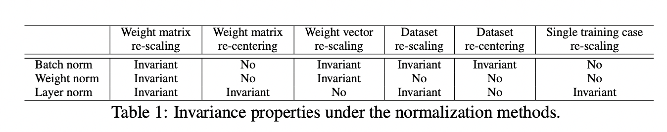
Weight re-scaling and re-centering

Let there be two sets of model parameters \(\theta, \theta^{\prime}\) whose weight matrices \(W, W^{\prime}\) differ by a scaling factor \(\delta\) and all of the incomping weights in \(W^{\prime}\) are also shifted by a constant vector \(\gamma\). That is \(W^{\prime} = \delta W + \mathbf{1}\gamma\). Under layer normalization:

\[\begin{aligned} \mathbf{h}^{\prime} &= f(\frac{\mathbf{g}}{\sigma^{\prime}} (\delta {W^{\prime}} + \mathbf{1} \gamma)^T \mathbf{x} - \mu) + \mathbf{b})\\ &= f(\frac{\mathbf{g}}{\sigma^{\prime}} (\delta {W^{\prime}}^T + \mathbf{1} \gamma^T)\mathbf{x} - \frac{1}{H}\sum_{i} (\delta{w_i^{\prime}}^T + \gamma^T)\mathbf{x})) + \mathbf{b})\\ &= f(\frac{\mathbf{g}}{\sigma} {W}^T \mathbf{x} - \mu) + \mathbf{b})\\ &= \mathbf{h} \end{aligned}\]

Data re-scaling and re-centering

Since the layer normalization only depends on the current input data point \(\mathbf{x}\), let \(\mathbf{x}^{\prime} = \delta \mathbf{x} + \lambda\), then:

\[\begin{aligned} h_i &= f(\frac{g_i}{\sigma^{\prime}} ({w_i^{\prime}}^T \mathbf{x}^{\prime} - \mu^{\prime}) + b_i)\\ &= f(\frac{g_i}{\sigma^{\prime}} ({w_i^{\prime}}^T \mathbf{x}^{\prime} - \frac{1}{H}\sum_{i} {w_i^{\prime}}^T\mathbf{x}^{\prime}) + b_i)\\ &= h_i \end{aligned}\]