Deep Deterministic Policy Gradient
Continuous Control with Deep Reinforcement Learning
Notations
A trajectory is defined as \((s_1, a_1, r_1, ...)\)
The initial state distribution: \(\rho (s_1)\)
Transition dynamics \(p(s_{t+1} | s_t, a_t)\)
Reward function \(r(s_t, a_t)\)
The return from a state is defined as the sum of discounted future reward:
\[R_t = \sum_{i=t}^{T} \gamma^{i - t} r(s_i, a_i)\]
The discounted state distribution following \(\pi\) is denoted as \(\rho^{\pi}\)
The action-value function:
\[Q^{\pi} (s_t, a_t) = E_{r_{i \geq t}, s_{i > t} \sim P, a_{i >t} \sim \pi} [R_t | s_t, a_t]\]
And the action-value function can be expanded using bellman equation:
\[Q^{\pi} (s_t, a_t) = E_{r_{t}, s_{t+1} \sim P} [r(s_t, a_t) + \gamma E_{a_{t+1} \sim \pi (\cdot | s_{t+1})}[Q^{\pi} (s_{t+1}, a_{t+1})] | s_t, a_t]\]
If we have deterministic policy \(\mu: S \rightarrow A\), we can remove the integral over next actions and have:
\[Q^{\mu} (s_t, a_t) = E_{r_{t}, s_{t+1} \sim P} [r(s_t, a_t) + \gamma Q^{\mu} (s_{t+1}, \mu(s_{t + 1})) | s_t, a_t]\]
This implies that we can learn \(Q^{\mu}\) off policy using state samples from another behavior policy \(\beta\).
The off policy loss for parameterized function approximators \(\theta^Q\) Bellman Residual Minimization is:
\[L(\theta^{Q}) = E_{s_t \sim \rho^\beta. a_t \sim \beta, r_t} [(Q(s_t, a_t | \theta^{Q}) - y_t)^2]\]
where:
\[y_t = r(s_t, a_t) + \gamma Q(s_{t+1}, \mu(s_{t+1}) | \theta^{Q})\]
The use of large, non-linear function approximators for learning value or action-value functions has often been avoided in the past since theoretical performance guarantees are impossible, and practically learning tends to be unstable.
The off policy deterministic policy gradient:
\[\nabla_{\theta^{\mu}} J \approx E_{s_{t} \sim \rho^{\beta}} [\nabla_{a} Q(s, a | \theta^Q) |_{s=s_t, a=\mu(s_t)}\nabla_{\theta_{\mu}} \mu(s | \theta^\mu) |_{s=s_t}]\]
As with Q learning, introducing non-linear function approximators means that convergence is no longer guaranteed for off-policy deterministic policy gradient.
Algorithm
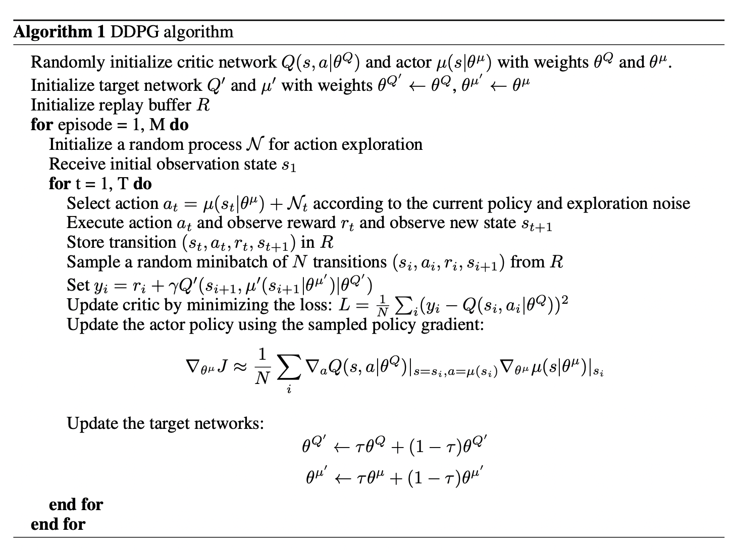
- Initialize:
- the weights \(\theta^Q\) for critic network \(Q\) and \(\theta^\mu\) for actor network \(\mu\)
- the weights \(\theta^{Q^{\prime}} \leftarrow \theta^{Q}\) for target critic \(Q^{\prime}\) and \(\theta^{\mu^{\prime}} \leftarrow \theta^{\mu}\) for target actor \(\mu^{\prime}\)
- the replay buffer \(R\)
- For each episode:
Initialize a random process \(\mathcal{N}_1, ....,\) for exploration
Observe initial state \(s_1 \sim \rho^{\mu^{\beta}} \;\;\;\;\;\;\;\;\;\;\;\) (remember we are learning off-policy)
For each timestep \(t = 1, ..., T\) in the episode:
Data generation
- \(a_t = \mu^{\beta} (s_t) = \mu (s_t | \theta^{\mu}) + \mathcal{N}_t \;\;\;\;\;\;\;\;\;\;\;\) (actions is selected with some noise)
- Observe \(s_{t+1}, r_t\) by following \(a_t\)
- Store \((s_t, a_t, r_t, s_{t+1})\) in \(R \;\;\;\;\;\;\;\;\;\;\;\) (for batch learning)
Now we evaluate \(Q^{\mu_{\theta}}\) and update \(\theta^{\mu}, \theta^{Q}\)
Sample a random minibatch of \(N\) transitions \((s_i, a_i, r_i, s_{i+1}) \;\;\;\;\;\;\;\;\;\;\;\) (for batch learning)
Calculate \(y_i = r_i + \gamma Q^{\prime} (s_{i+1}, \mu^{\prime} (s_{i+1}))\;\;\;\;\;\;\;\;\;\;\;\) (\(\hat{T}^{\mu^{\prime}} Q^{\prime}\))
Update critic by minimizing the loss \(L = \frac{1}{N} \sum_{i} (Q(s_i, a_i) - y_i)^2 \;\;\;\;\;\;\;\;\;\;\;\) (update for several times, to have a better estimate of \(\hat{T}^{\mu^{\prime}} Q^{\prime}\))
Update the actor policy using the sampled policy gradient:
\[\frac{1}{N} \sum_i \nabla_{a} Q(s, a) |_{s=s_i, a=\mu(s_i)} \nabla_{\theta^{\mu}} \mu(s_i)\]
Update the target critic and target actor:
\[\theta^{Q^{\prime}} \leftarrow \tau \theta^{Q} + (1 - \tau) \theta^{Q^{\prime}}\] \[\theta^{\mu^{\prime}} \leftarrow \tau \theta^{\mu} + (1 - \tau) \theta^{\mu^{\prime}}\]
Features:
Use replay buffer to address correlated samples. Because DDPG is an off-policy algorithm, the replay buffer can be large, allowing the algorithm to benefit from learning across a set of uncorrelated transitions.
Similar to target network in DQN, a soft target updates rather than directly copying the weights is used. We create a copy of the actor and critic networks, \(Q^{\prime} (s, a | \theta^{Q^{\prime}})\) and \(\mu^{\prime} (s | \theta^{\mu^{\prime}})\). Notice here, the target is calculated using these delayed parameters. One problem with this is that:
\[E[r(s_t, a_t) + \gamma Q^{\prime} (s, \mu^{\prime} (s_{t+1} | \theta^{\mu^{\prime}}) | \theta^{Q^{\prime}})] = E[\hat{T}^{\mu^{\prime}} Q^{\prime} (s, a)] = T^{\mu^{\prime}} Q^{\prime} (s, a)\]
So, if we minimize the square loss of the critic w.r.t this target for some iterations, then follow the approximate value iteration, we end up evaluating \(Q^{\mu^{\prime}} (s, a)\).
The weights of these target networks are then updated by having them slowly track the learned networks: \(\theta^{\prime} \leftarrow (1 - \tau) \theta^{\prime} + \theta\) (stochastic approximation of mean of \(\theta\)) with \(\tau << 1\). This means that the target values are constrained to change slowly, greatly improving the stability of learning. The authors found that having both a delayed \(\mu^{\prime}\) and a delayed \(Q^{\prime}\) was required to have stable \(y_t\) in order to consistently train the critic without divergence.
In low dimensional feature vector observation space, Batch Normalization is used to normalize each dimension across the samples in a mini-batch to have unit mean and variance. A running average of mean and variance is maintained in training time and used in test time in this case evaluation or exploration. This technique is applied on the state input and all layers of the \(\mu\) network and all layers of the \(Q\) network prior to the action input. This help with the learning speed and scalability across different envs and units.
Exploration problem is resolved by having a separate exploration policy \(\mu^{\prime}\) (different from target network \(\mu^{\prime} (s | \theta^{\mu^{\prime}})\)) by adding noise sampled from a noise process \(N\) to our current actor policy:
\[\mu^{\prime} (s_t) = \mu (s_t | \theta_t^{\mu}) + \mathcal{N}\]
This \(N\) can be chosen to suit the environment.