PPO
Proximal Policy Optimization Algorithms
Notations and Backgrounds
Policy gradient estimator
\[\hat{g} = \hat{E}_t [\nabla_{\theta} \log \pi_{\theta} (a_t | s_t) \hat{A_t}]\]
Where, \(\pi_{\theta}\) is the stochastic policy and \(\hat{A_t}\) is an estimate of advantage function at timestep \(t\). The expectation here \(\hat{E}_t\) indicates the empirical average over a finite batch of samples, in an algorithm that alternates between sampling and optimization.
\(\hat{g}\) is obtained by differentiating the objective
\[L^{PG} (\theta) = \hat{E}_t [\log \pi_{\theta} (a_t | s_t) \hat{A_t}]\]
While it is appealing to perform multiple steps of optimization on this loss \(L^{PG} (\theta)\) (reuse the same samples to update \(\theta\)), using the same trajectory, doing so is not well-justi ed, and empirically it often leads to destructively large policy updates.
Trust Region Methods
The optimization problem is defined as:
\[\begin{aligned} \max_{\theta} \quad & \hat{E}_{s \sim \rho_{\theta_{old}} (\cdot), \; a \sim \pi_{\theta_{old}}(\cdot | s)} [\frac{\pi_{\theta} (a | s)}{\pi_{\theta_{old}} (a | s)} \hat{A}_{\theta_{old}} (s, a)]\\ \textrm{s.t.} \quad & \hat{E}_{s \sim \rho_{\theta_{old}} (\cdot)}[D_{KL} (\pi_{\theta_{old}} (\cdot | s) || \pi_{\theta} (\cdot | s))] \leq \delta \end{aligned}\]It is also possible to remove the hard constraint and convert the problem to an unconstrained objective:
\[\begin{aligned} \max_{\theta} \quad & \hat{E}_{s \sim \rho_{\theta_{old}} (\cdot), \; a \sim \pi_{\theta_{old}}(\cdot | s)} [\frac{\pi_{\theta} (a | s)}{\pi_{\theta_{old}} (a | s)} \hat{A}_{\theta_{old}} (s, a) - \beta D_{KL}[\pi_{\theta_{old}} (\cdot | s) || \pi_{\theta} (\cdot | s))]]\\ \end{aligned}\]The problem with this objective is that, the penalty prefers small steps, so it is very hard to choose an appropriate \(\beta\) that performs well across different problems or even within a single problem where the characteristics change over the course of learning.
Clipped Surrogate Objective
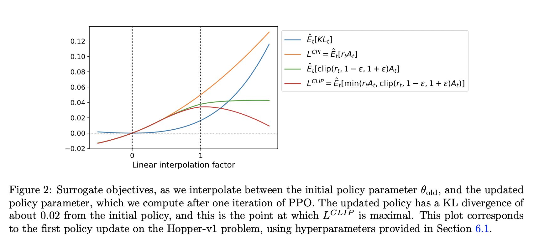
Let \(r_t (\theta)\) denotes the probability ratio \(r_t (\theta) = \frac{\pi_{\theta} (a_t | s_t)}{\pi_{\theta_{old}} (a_t | s_t)}\), so \(r (\theta_{old}) = 1\). The above unconstrained TRPO objective without penalty becomes:
\[L^{CPI} (\theta) = \hat{E}_{s \sim \rho_{\theta_{old}} (\cdot), \; a \sim \pi_{\theta_{old}} (\cdot | s)} [r_{t} (\theta) \hat{A}_{\theta_{old}} (s, a)]\]
Without the penalty, the step size can be super big maximizing \(L^{CPI}\), thus, we can add penalty to the changes to the policy that move \(r_t (\theta)\) away from 1 (make big updates or take big step)
The main objective is then:
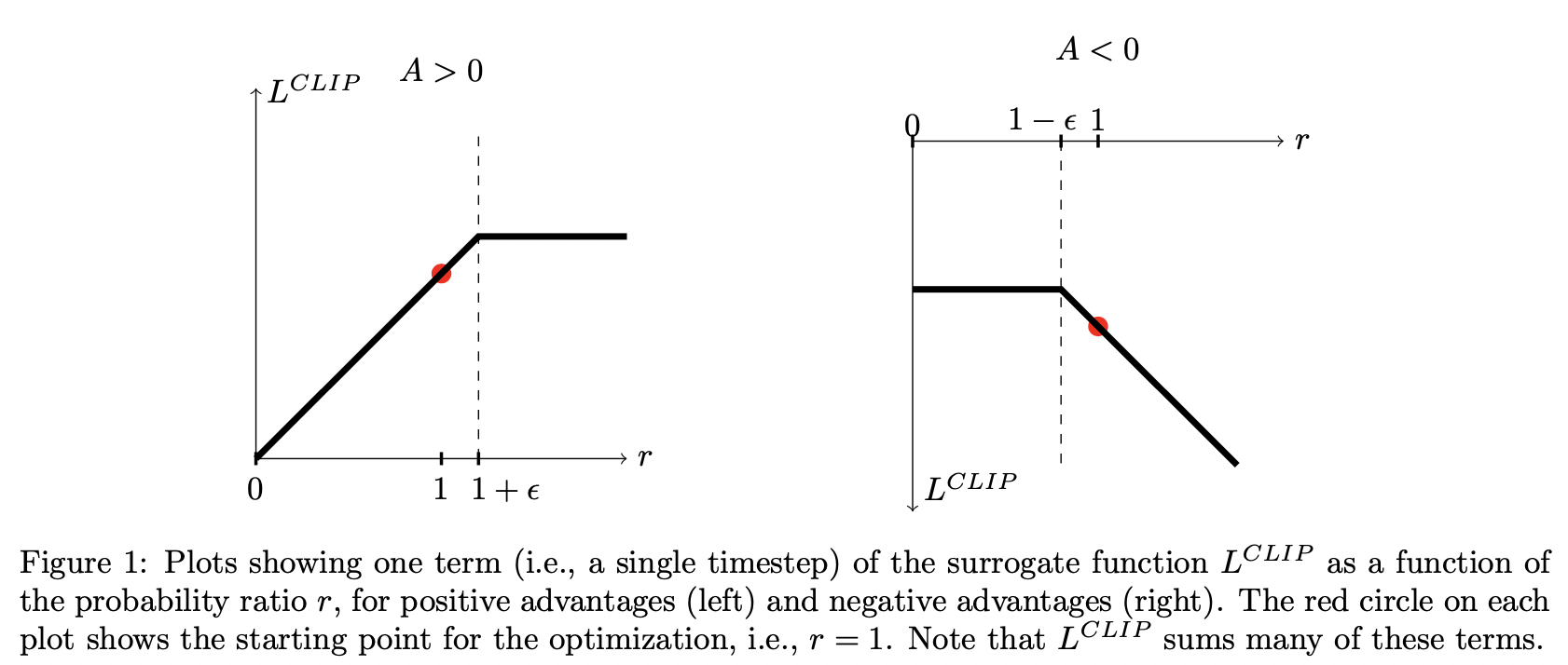
\[L^{CLIP} (\theta) = \hat{E}_{s \sim \rho_{\theta_{old}} (\cdot), \; a \sim \pi_{\theta_{old}} (\cdot | s)} [\min (r_{t} (\theta) \hat{A}_{\theta_{old}} (s, a), \text{clip}(r_t(\theta), 1 - \epsilon, 1 + \epsilon)\hat{A}_{\theta_{old}} (s, a))]\]
Notice here, the clipped objective gives a lower bound of the unclipped objective, to see this:
- If \(A_t < 0\), then one way to maximize the objective is to make \(r_t\) very small, then we will have a really large step size, However, with clipped objective, the largest change is clipped to \(1 - \epsilon\)
- If \(A_t > 0\), then one way to maximize the objective is to make \(r_t\) very large, then we will have a really large step size. However, with clipped objective, the largest change is clipped to \(1 + \epsilon\)
At the same time, the minimum gives the above behavior to account for \(A_t > 0, A_t < 0\) situation.
Adaptive KL Penalty Coefficient
Another approach, which can be used as an alternative to the clipped surrogate objective, or in additional to it is to use a penalty on KL divergence \(d_{targ}\) each policy update. In practice, KL performs worse than the clipped surrogate objective.
In the simplest instantiation of this algorithm, the following steps are used in each policy update:
Using several epochs of mini-batch SGD, optimizing the KL-penalized objective:
\[L^{KLPEN} (\theta) = \hat{E}_t [\frac{\pi_\theta (a_t | s_t)}{\pi_{\theta_{old}} (a_t | s_t)} \hat{A}_t - \beta_t D_{KL} (\pi_{\theta_{old}} (\cdot | s) || \pi_{\theta} (\cdot | s))]\]
Compute and update \(\theta_{t+1}\):
\[d = \hat{E}_t [\beta_t D_{KL} (\pi_{\theta_{old}} (\cdot | s) || \pi_{\theta} (\cdot | s))]\]
- If \(d < d_{targ} \;/\; 1.5, \quad \beta_{t + 1} \leftarrow \beta_{t} \;/\; 2\)
- If \(d > d_{targ} * 1.5, \quad \beta_{t + 1} \leftarrow \beta_{t} * 2\)
\(\beta_{t + 1}\) is used in the next policy update. The algorithm is not very sensitive to the choice of \(2\) and \(1.5\) above. The initial value of \(\beta\) is another hyperparameter but is not important in practice.
Algorithm
The advantage function can be estimated using a separate value function \(V(x)\), or a shared parameter value and policy network can be used. If the parameters are shared between policy network and value network, we need to modify the objective by adding the value loss negative value function loss \(- L^{VF} (\theta)\) and maybe an entropy term to promote exploration:
\[L^{CLIP + VF + S} (\theta) = \hat{E} [L_t^{CLIP} (\theta) - c_1 L_t^{VF} (\theta) + c_2 S[\pi_{\theta}] (s_t)]\]
Where, \(c_1, c_2\) are two coefficients, \(S[\pi_{\theta}] (s_t)\) is the entropy bonus on \(s_t\) and \(L_t^{VF} = \|V_{\theta} - V_t^{targ}\|^2\) is the square loss.
One style of advantage estimate is n-step TD estimate:
\[\hat{A}_t = r_t + \gamma r_{t+1} + .... + \gamma^{T-t+1} r_{T-1} + \gamma^{T-t} V(s_T) - V(s_t)\]
Where \(t\) specifies the time index in \([0, T]\), within a given length-\(T\) trajectory segment. Using this idea, we can use a truncated version of generalized advantage estimation:
\[\hat{A}_t = \delta_t + \gamma \lambda \delta_{t+1} + .... + \lambda \gamma^{T-t+1}\delta_{T-1}\]
\[\delta_t = r_t + \gamma V(s_{t+1}) - V(s_t)\]
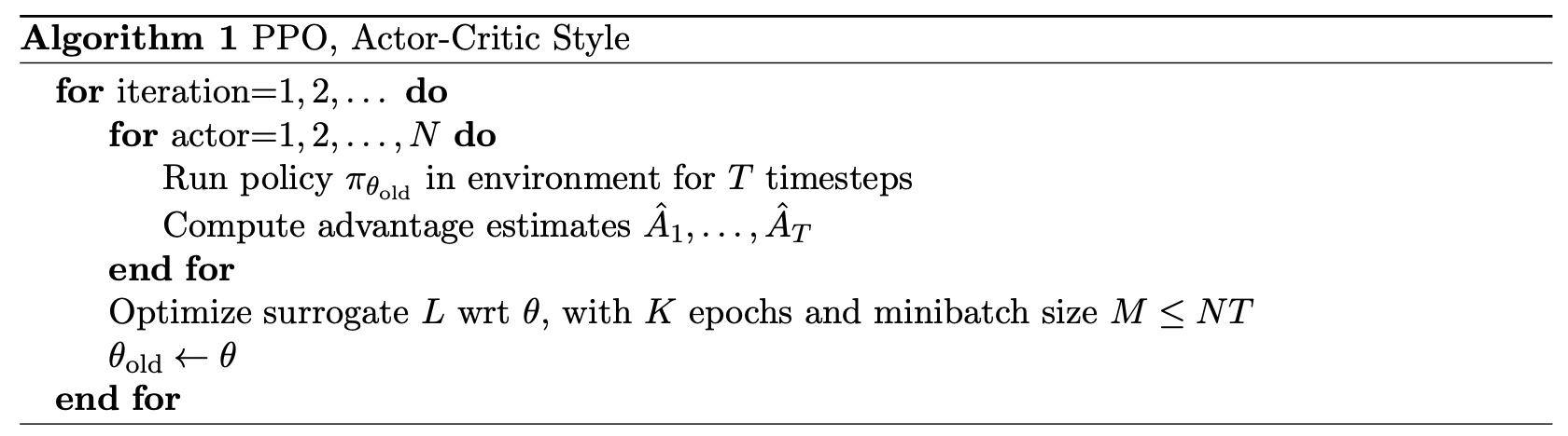
A PPO algorithm that uses fixed-length trajectory segments is shown above. Each iteration, each \(N\) parallel actors collect \(T\) timesteps of data. Then we construct the surrogate loss on these \(NT\) timesteps of data and optimize it with mini-batch SGD for \(K\) epochs.
Implementation
One implementation from parl
1 | # Copyright (c) 2021 PaddlePaddle Authors. All Rights Reserved. |