TRPO

Trust Region Policy Optimization

Notations

\(A_{\pi}, A^{\pi}\) are the same, just some mismatch in the notations during writing, same for \(V, Q\) :<

Consider an infinite-horizon discounted MDP, defined by the tuple \((S, A, P, r, \rho_0, \gamma)\). \(S\) is finite set of states and \(A\) is finite set of actions $r: S $.

The expected discounted return over initial state distribution \(\rho_0\) (performance measure):

\[\eta (\pi) = E_{s_0, a_0, ...} [\sum^{\infty}_{t=0} \gamma^t r(s_t)]\]

Where \(s_0 \sim \rho_0, a_t \sim \pi (\cdot | s_t), s_{t+1} \sim P(\cdot | s_t, a_t)\)

Value functions:

\[Q_{\pi} (s_t, a_t) = E_{s_{t+1}, a_{t+1}, ..}[\sum^{\infty}_{l=0} \gamma^{l} r(s_{t+l}) | S_t=s_t, A_t=a_t]\]

\[V_{\pi} (s_t) = E_{a_{t}, s_{t+1}, a_{t+1}, ..}[\sum^{\infty}_{l=0} \gamma^{l} r(s_{t+l}) | S_t=s_t]\]

The advantage:

\[A(s, a) = Q_{\pi} (s, a) - V_{\pi} (s)\]

The discounted future state distribution (unormalized):

\[\rho_{\pi} (s) = \lim_{t \rightarrow \infty} \sum_{t} \rho(s_0) \gamma^t P(s_0 \rightarrow s; t, \pi)\]

The difference in policy performance as expected advantages over states and actions

Given two policies \(\pi, \tilde{\pi}\), the performance of \(\tilde{\pi}\):

\[\eta (\tilde{\pi}) = \eta(\pi) + E_{\tau \sim \tilde{\pi}} [\sum^{\infty}_{t = 0} \gamma^t A_{\pi} (s_t, a_t)]\]

Proof

First:

\[\begin{aligned} E_{s^{\prime}} [r(s) + \gamma V^{\pi} (s^{\prime}) - V^{\pi} (s) | s, a] &= E_{s^{\prime}} [r(s) + \gamma V^{\pi} (s^{\prime}) | s, a] - V^{\pi} (s)\\ &= r(s) + \gamma \int_{s^{\prime}, a^{\prime}} P(ds^{\prime} | s, a)\pi(da^{\prime} | s^{\prime}) Q^{\pi} (s^{\prime}, a^{\prime}) - V^{\pi} (s)\\ &= Q^{\pi}(s, a) - V^{\prime} (s)\\ &= A_{\pi}(s, a) \end{aligned}\]

Thus:

\[\begin{aligned} E_{\tau \sim \tilde{\pi}} [\sum^{\infty}_{t=0} \gamma^t A_{\pi} (s_t, a_t)] &= E_{\tau \sim \tilde{\pi}} [\sum^{\infty}_{t=0} \gamma^t E_{s_{t+1}} [r(s_t) + \gamma V^{\pi} (s_{t+1}) - V^{\pi} (s_t) | s_t, a_t]]\\ &= E_{\tau \sim \tilde{\pi}} [\sum^{\infty}_{t=0} \gamma^t (r(s_t) + V^{\pi} (s_{t+1}) - V^{\pi} (s_t))]\\ &= E_{\tau \sim \tilde{\pi}} [\sum^{\infty}_{t=0} \gamma^t(\gamma V^{\pi}(s_{t+1}) - V^{\pi}(s_{t})) + \sum^{\infty}_{t=0} \gamma^t r(s_t)]\\ &= E_{\tau \sim \tilde{\pi}} [ - V^{\pi}(s_{0}) + \sum^{\infty}_{t=0} \gamma^t r(s_t)]\\ &= E_{s_0} [- V^{\pi}(s_{0})] + E_{\tau \sim \tilde{\pi}} [\sum^{\infty}_{t=0} \gamma^t r(s_t)]\\ &= - \eta (\pi) + \eta (\tilde{\pi}) \end{aligned}\]

The improvement can be written as per timestep advantage.

At the same time, the improvement can rewrite using discounted future state distribution (unormalized):

\[\begin{aligned} \eta (\tilde{\pi}) &= \eta (\pi) + E_{\tau \sim \tilde{\pi}} [\sum^{\infty}_{t=0} \gamma^t A_{\pi} (s_t, a_t)]\\ &= \eta (\pi) + \sum^{\infty}_{t=0} \gamma^t E_{\tau \sim \tilde{\pi}} [A_{\pi} (s_t, a_t)]\\ &= \eta (\pi) + \sum^{\infty}_{t=0} \gamma^t E_{s_t, a_t} [A_{\pi} (s_t, a_t)]\\ &= \eta (\pi) + \sum^{\infty}_{t=0} \gamma^t \sum_{s_{t}, a_{t}, s_0} \rho(s_0) P(s_0 \rightarrow s_t; t, \tilde{\pi}) \tilde{\pi}(a_t|s_t) A_{\pi} (s_t, a_t) \\ &= \eta (\pi) + \sum_{s_{t}, a_{t}, s_{0}} \sum^{\infty}_{t=0} \gamma^t \rho(s_0) P(s_0 \rightarrow s_t; t, \tilde{\pi}) \tilde{\pi}(a_t|s_t) A_{\pi} (s_t, a_t) \\ &= \eta (\pi) + \sum_{s_{t}} \rho_{\tilde{\pi}} (s_t) \sum_{a_{t}} \tilde{\pi}(a_t|s_t) A_{\pi}(s_t, a_t) \end{aligned}\]

This equation implies that any policy update \(\pi \rightarrow \tilde{\pi}\) that has non-negative expected advantage over actions at every state \(s_t\) is guaranteed to increase the policy performance measure \(\eta\) or leave it constant

Local Approximation to \(\eta\)

In the approximate setting, it will typically be unavoidable, due to estimation error and approximation error that there will be some states with expected advantage over actions less than 0:

\[E_{a \sim \tilde{\pi} (\cdot | s)}[A_{\pi} (s, a) | s] < 0\]

At the same time, the expectation also depends on \(\rho^{\tilde{\pi}}\) which makes it difficult to optimize directly (the future state distribution is unknown, we cannot sample from unknown distribution), instead, we can use following local approximation to \(\eta\):

\[\begin{aligned} L_{\pi} (\tilde{\pi}) &= \eta (\pi) + \underbrace{\sum_{s_t} \rho_{\pi} (s_t)}_{\text{we replace unnormalized state distribution}} \sum_{a_t} \tilde{\pi}(a_t|s_t) [A_{\pi}(s_t, a_t)]\\ &= \eta (\pi) + \frac{1}{1 - \gamma}E_{s_t \sim \rho^{\pi} (\cdot), a_t \sim \tilde{\pi}(\cdot | s_t)} [A^{\pi}(s_t, a_t)]\\ &= \eta (\pi) + \frac{1}{1 - \gamma}\mathbb{A}_{\pi} (\tilde{\pi}) \end{aligned}\]

We now ignore the change in state distribution due to the changes in the policy. If \(\pi\) is parametrized by \(\theta\), then:

\[L_{\pi_\theta} (\pi_{\theta}) = \eta (\pi_{\theta}) + \underbrace{ \sum_{s_t} \rho_{\pi_{\theta}} (s_t) \sum_{a_t} \pi(a_t|s_t) [A_{\pi_{\theta}}(s_t, a_t)]}_{E_{a \sim \pi}[A_{\pi_{\theta}} (s, a) | s] = 0} = \eta (\pi_{\theta})\]

Consider a small update on \(\theta\) such that \(\pi_{\theta_{new}} = (1 - \alpha) \pi_{\theta} + \alpha \pi_{\theta^{\prime}}\), then:

\[\begin{aligned} \nabla_{\alpha} \eta (\pi_{\theta_{new}}) |_{\alpha = 0} &= \nabla_{\pi_{\theta_{new}}} \eta (\pi_{\theta_{new}}) \nabla_{\alpha} \pi_{\theta_{new}} |_{\pi_{\theta_{new}} = \pi_{\theta}}\\ &= \sum_{s_t, a_t} \rho^{\pi_{\theta_{new}}} (s_t) \nabla_{\pi_{\theta_{new}}} \pi_{\theta_{new}} (a_t | s_t) (\pi_{\theta^{\prime}} (a_t | s_t) - \pi_{\theta} (a_t | s_t)) A^{\pi_{\theta_{new}}}(s_t, a_t)|_{\pi_{\theta_{new}} = \pi_{\theta}}\\ &= \sum_{s_t, a_t} \rho^{\pi_{\theta}} (s_t) \pi_{\theta^{\prime}} (a_t | s_t) A^{\pi_{\theta}}(s_t, a_t) - \sum_{s_t, a_t} \rho^{\pi_{\theta}} (s_t) \pi_{\theta} (a_t | s_t) A(s_t, a_t)\\ &= \sum_{s_t, a_t} \rho^{\pi_{\theta}} (s_t) \pi_{\theta^{\prime}} (a_t | s_t) A^{\pi_{\theta}}(s_t, a_t) - \sum_{s_t} \rho^{\pi_{\theta}} (s_t) \sum_{a_t} \pi_{\theta} (a_t | s_t) Q^{\pi_{\theta}}(s_t, a_t) - V^{\pi_{\theta}} (s_t)\\ &= \sum_{s_t, a_t} \rho^{\pi_{\theta}} (s_t) \pi_{\theta^{\prime}} (a_t | s_t) A^{\pi_{\theta}}(s_t, a_t)\\ &= \frac{1}{1 - \gamma}\sum_{s_t, a_t} (1 - \gamma)\rho^{\pi_{\theta}} (s_t) \pi_{\theta^{\prime}} (a_t | s_t) A^{\pi_{\theta}}(s_t, a_t)\\ &= \frac{1}{1 - \gamma} E_{s_t \sim \rho^{\pi_{\theta}} (\cdot), a_t \sim \pi_{\theta^{\prime}}(\cdot | s_t)} [A^{\pi_{\theta}}(s_t, a_t)]\\ &= \frac{1}{1 - \gamma}\mathbb{A}_{\pi_{\theta}} (\pi_{\theta^{\prime}}) \end{aligned}\]

By the same insight, we can conclude that \(\alpha A_{\pi_{\theta}} (\pi_{\theta^\prime}) = A_{\pi_{\theta}} (\pi_{\theta_{new}})\). Using Talyor's expansion and above first order results, we can see that the change in \(\Delta \eta\):

\[\eta (\pi_{\theta_{new}}) - \eta (\pi_{\theta}) \geq \frac{1}{1 - \gamma}\mathbb{A}_{\pi_{\theta}} (\pi_{\theta_{new}}) - O(\alpha^2)\]

\[\implies \eta (\pi_{\theta_{new}}) \geq L_{\pi_{\theta}} (\pi_{\theta_{new}}) - O(\alpha^2)\]

These results imply that a sufficiently small step \(\alpha\), \(\pi_{\theta} \rightarrow \tilde{\pi}\) that improves \(L_{\pi_{\theta}}\) will also improve \(\eta\). However, it does not tell us how big of the step to take. To address this issue, some previous works proposed:

\[\pi_{new} (a | s) = (1 - \alpha) \pi_{old} (a | s) + \alpha \pi^{\prime} (a | s)\]

Where \(\pi^{\prime} = \arg\max_{\pi^{\prime}} L_{\pi_{old}} (\pi^{\prime})\)

They also derive the lower bound:

\[\eta (\pi_{new}) \geq L_{\pi_{old}} (\pi_{new}) - \frac{2 \epsilon \gamma}{(1 - \gamma)^2} \alpha^2\]

Where \(\epsilon = \max_{s} | E_{a \sim \pi^{\prime}} [A_{\pi} (s, a)]|\)

However, this bound only applies to the above policy update rule and is restrictive in practice.

Monotonic Improvement Guarantee for General Stochastic Policies

We can extend the above lower bound to more general case stochastic policies by replacing \(\alpha\) with some distance measurement between \(\pi\) and \(\tilde{\pi}\) and change \(\epsilon\) accordingly. The particular distance measure in this case is total variation divergence, for discrete probability distributions \(p, q\)

\[D_{TV} (p || q) = \frac{1}{2} \sum_{i} |p_i - q_i|\]

Define the maximum distance to be the maximum total variation divergence over states:

\[D^{\max}_{TV} (\pi, \tilde{\pi}) = \max_{s} D_{TV} (\pi(\cdot | s) || \tilde{\pi} (\cdot | s))\]

Notice that the relationship between KL divergence and total variation divergence:

\[D_{TV} (p || q)^2 \leq D_{KL} (p || q)\]

Let:

\[D^{\max}_{KL} (\pi, \tilde{\pi}) = \max_{s} D_{KL} (\pi(\cdot | s) || \tilde{\pi} (\cdot | s)) \geq D^{\max}_{TV} (\pi, \tilde{\pi})\]

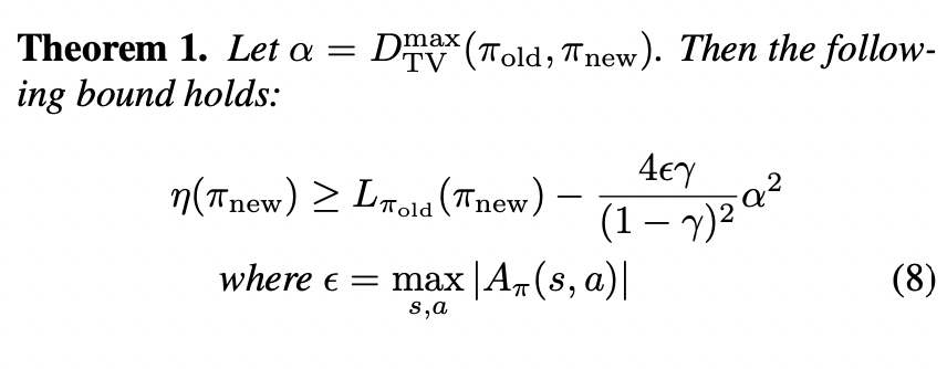
Then, the lower bound becomes:

\[\eta (\tilde{\pi}) \geq L_{\pi} (\tilde{\pi}) - C D^{\max}_{TV} (\pi, \tilde{\pi})^2 \geq L_{\pi} (\tilde{\pi}) - C D^{\max}_{KL} (\pi, \tilde{\pi})\]

Where \(C = \frac{4\epsilon \gamma}{(1 - \gamma)^2}\), \(\epsilon = \max_{s, a} |A_{\pi} (s, a)|\)

Population Version of the Algorithm

The population version of the algorithm assumes exact evaluation of the advantage function:

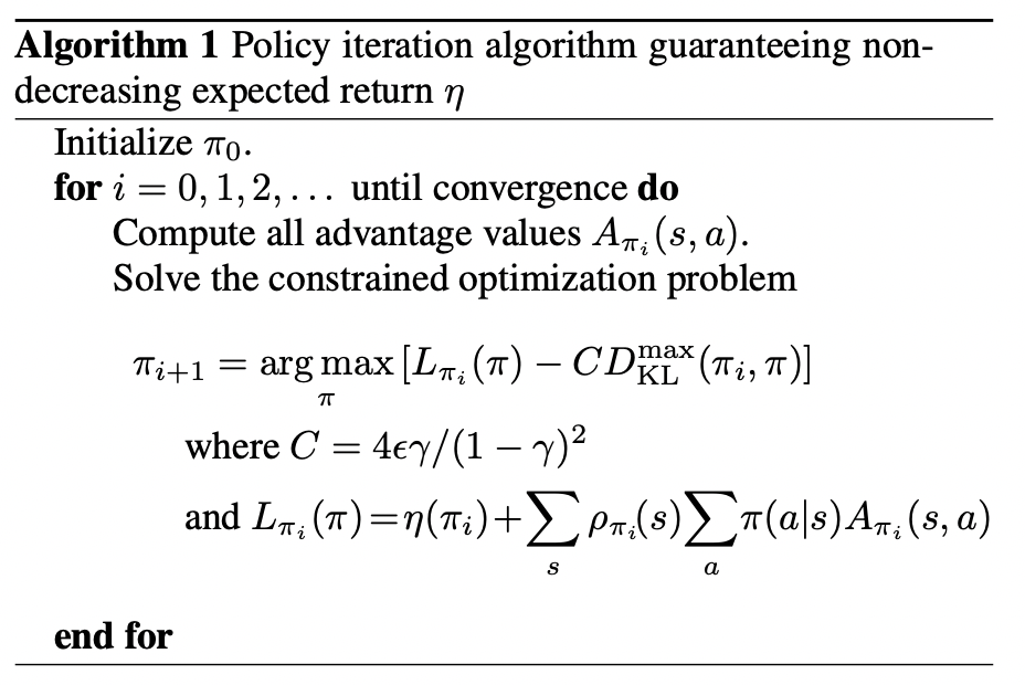
We can see that the algorithm generate monotonically improved sequence of performance measure \(\eta (\pi_0) \leq \eta (\pi_1) \leq \eta (\pi_2) \leq ...\). To see this, let \(M_i (\pi) = L_{\pi_i} (\pi) - CD^{\max}_{KL} (\pi, \tilde{\pi})\):

\[\begin{aligned} \eta (\pi_{i + 1}) &\geq M_i (\pi_{i + 1})\\ \eta (\pi_{i}) &= M_i (\pi_i)\\ \eta (\pi_{i + 1}) - \eta (\pi_{i}) &\geq M_i (\pi_{i + 1}) - M_i (\pi_i) \end{aligned}\]

Since we are maximizing \(M_i (\pi_i)\) at each iteration \(\implies M_i (\pi_i) \geq M_i (\pi_i)\). The improvement is non-decreasing.

Optimization of Parameterized Policies

Since we are parameterizing policy by \(\theta\), some additional notations are used in place of the \(\pi\)

\[\eta (\theta) := \eta(\pi_\theta) \;\;\;\;\; L_{\theta}(\tilde{\theta}) := L_{\pi_{\theta}} (\pi_{\tilde{\theta}}) \;\;\;\;\; D_{KL} (\theta || \tilde{\theta}) := D_{KL} (\pi_{\theta} || \tilde{\pi}_{\theta})\]

\(\theta_{old}\) is used to denote the previous policy parameters that we want to improve upon.

The previous theorem suggest that, if we maximize:

\[\max_{\theta} \quad [L_{\theta_{old}} (\theta) - CD^{\max}_{KL} (\theta_{old}, \theta)]\]

Then we are guaranteed to improve our policy with equality when \(\theta_{old} = \theta\).

However, since the penalty term is \(CD^{\max}_{KL} (\theta_{old}, \theta)\) which means smaller change in policy distribution is preferred. If we maximize this objective with penalty coefficient \(C\), we will end up with very small step-size. One way to take larger step size is to use a constraint on the KL divergence between the new policy and the old policy (Trust Region Constraint):

\[\begin{aligned} \max_{\theta} \quad & L_{\theta_{old}} (\theta)\\ \textrm{s.t.} \quad & D^{\max}_{KL} (\theta_{old}, \theta) \leq \delta \end{aligned}\]

This optimization problem is impractical to solve due to large number of constraints, but we can use a heuristic approximation which considers the average KL divergence:

\[\bar{D}^\rho_{KL} (\theta_1, \theta_2) := E_{s \sim \rho}[D_{KL} (\pi_{\theta_1} (\cdot | s) || \pi_{\theta_2} (\cdot | s))]\]

Then the optimization problem can be rewritten as:

\[\begin{aligned} \max_{\theta} \quad & L_{\theta_{old}} (\theta)\\ \textrm{s.t.} \quad & \bar{D}^{\rho_{\theta_{old}}}_{KL} (\theta_1, \theta_2) \leq \delta \end{aligned}\]

Sample-Based Algorithm

The above population version optimization problem can be approximated using MC simulation:

\[\begin{aligned} \max_{\theta} \quad & E_{s \sim \rho_{\theta_{old}} (\cdot), \; a \sim q (\cdot | s)} [\frac{\pi_{\theta} (a | s)}{q (a | s)} \hat{Q}_{\theta_{old}} (s, a)]\\ \textrm{s.t.} \quad & E_{s \sim \rho_{\theta_{old}} (\cdot)}[D_{KL} (\pi_{\theta_{old}} (\cdot | s) || \pi_{\theta} (\cdot | s))] \leq \delta \end{aligned}\]

1. Drop constant \(\eta (\theta_{old})\) from the objective
2. Replace advantage \(A_{\theta_{old}}\) with \(Q_{\theta_{old}}\), because \(V_{\pi_{old}} (s)\) only affects the value at each state by a constant (does not depend on policy).
3. Place sampling of action \(a\) by an importance sampling, we can use one trajectory to sample both actions and states if \(q = \pi_{\theta_{old}}\).
4. Substitute an estimate \(\hat{Q}_{\theta_{old}}\) for \(Q_{\theta_{old}}\)

Collecting Samples (Single Path)

In this estimation procedure, we collect a sequence of states by sampling \(s_0 \sim \rho_0\), then simulating the trajectory \(\tau = (s_0, a_1, s_1, a_2, ..., s_T)\) by following \(\pi_{old}\), and discount each estimate of the expectation by \(\gamma^t\), then the samples of \(s_i\) would be from the discounted state distribution. Then, we use discounted return \(G\) to be the unbiased estimator of \(Q_{\theta_{old}}\), that is, \(\hat{Q}_{\theta_{old}} = G\)

Collecting Samples (Vine)

Ignored Here

Conclusions

1. The theory justifies optimizing a surrogate objective with a penalty on step size (KL divergence) would guarantee policy improvement. However, the large penalty coefficient C leads to prohibitively small steps, so we relax the penalty by converting the problem to a constraint optimization problem with hard threshold on the step size \(\alpha\) which is defined as the average DL divergence. This divergence is easier for numerical optimization and estimation than max KL divergence.

2. The theory in this paper ignores estimation error for the advantage function.

Reference

https://ieor8100.github.io/rl/docs/Lecture%207%20-Approximate%20RL.pdf

https://people.eecs.berkeley.edu/~pabbeel/cs287-fa09/readings/KakadeLangford-icml2002.pdf