Alex Net
ImageNet Classification with Deep Convolutional Neural Networks
The dataset, Image preprocessing
ImageNet is a dataset of over 15 million labeled high-resolutoin images. It consists of variable-resolution images, while the network requires a constant input dimensionality. Therefore, we down-sampled the images to a fixed resolution of \(256 \times 256\). Given a rectangular image, we first rescaled the image such that the shorter side was of length 256, and then cropped out the central \(256 \times 256\) patch from the resulting image. We did not pre-process the images in any other way, except for subtracting the mean activity over the training set for each pixel (normalize each input pixel). So we trained our network on the centered raw RGB values of the pixels.
The Architecture
ReLU Nonlinearity
tanh and other saturating nonlinearities are much slower than the non-saturating nonlinearity \(f(x) = max(0, x)\). DNN with ReLUs train several times faster than their equivalents with tanh units.
Training on Multiple GPUs
We split half of the kernels (neurons) on each GPU, with one additional trick: the GPUs communicate only in certain layers. This means that, for examples, the kernels of layer 3 take input form all kernel maps in layer 2. However, kernels in layer 4 take input only from those kernel maps in layer 3 which reside on the same GPU. This allows us to precisely tune the amount of communication until it is an acceptable fraction of the amount of computation.
Local Response Normalization
Denoting by \(a^{i}_{x, y}\) the activity of a neuron computed by applying kernel \(i\) at position \((x, y)\) and then applying the ReLU nonlinearity, the response-normalized activity \(b^i_{x,y}\) is given by the expression:
\[b^{i}_{x, y} = \frac{a^{i}_{(x, y)}}{(k + \alpha \sum_{j=\max(0 , \frac{i - n}{2})}^{\min(N - 1, \frac{i + n}{2})}(a^{i}_{(x, y)})^2)^\beta}\]
Where the sum runs over \(N\) adjacent kernel maps at the same spatial position, and \(N\) is the total number of kernels in the layer. This normalization is applied after applying the ReLU nonlinearity in certain layers.
Overlapping Pooling
Pooling layers in CNNs summarize the outputs of neurons in the same kernel map. Traditionally, the pooling units do not overlap. To be more precise, a pooling layer can be though of as consisting of a grid of pooling units spaced \(s\) pixels apart, each summarizing a neighborhood of size \(z \times z\) centered at the location of the pooling unit. If we set \(s = z\), we obtain traditional local pooling. If \(s < z\), we obtain overlapping pooling. This is used in the network. We generally observe during training that models with overlapping pooling find it slightly more difficult to overfit.
Reduce Overfitting
Data Augmentation
Two distinct forms of data augmentation:
Generating image translations and horizontal reflections. We do this by extracting random \(227 \times 227\) patches, and their horizontal reflections from the \(256 \times 256\) images and training our network on these extracted patches. At the test time, the network makes a prediction by extracting 5 \(227 \times 227\) patches (4 corner patches and 1 center patch) as well as their horizontal reflections and average the predictions made by the network's softmax layer on the ten patches.
Altering the intensities of the RGB channels in training images. Specifically, we perform PCA on the set of RGB pixel values throughout the imageNet training set. For each training image, we add multiples of the found principal components with magnitudes proportional to the corresponding eigenvalues times a random variable drawn from a Gaussian with mean zero and std 0.1.
Dropout
Model aggregation using dropout. Attest time, we use all the neurons but multiply their outputs by 0.5, which is a reasonable approximation to taking the geometric mean of the predictive distributions produced by the exponentially-many dropout networks.
We use dropout in the first two fully-connected layers. Without dropout, our network exhibits substantial overfitting. Dropout roughly doubles the number of iterations required to converge.
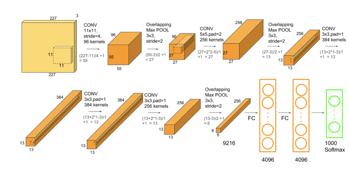
Overall Architecture
The net contains eight layers with weights, the first five are convolutional and the remaining three are full-connected. The output of the last fully-connected layer is fed to a 1000-way softmax which produces a distribution over the 1000 class labels. The network maximizes the multinomial logistic regression objective (-cross entropy), which is equaivalent to maximizing the average across training cases of the log-probability of the correct label under the prediction distribution.
The kernels of the second, fourth and fifth convolutional layers are connected only to those kernel maps in the previous layer which reside on the same GPU. The kernels of the third convolutional layer are connected to all kernel maps in the second layer. The neurons in the fully connected layers are connected to all neurons in the previous layer. Normalization layers follow the first and second convolutional layers. Max-pooling layers, of the kind with overlapping, follow both normalization layers and the fifth convolutional layer.
The first convolutional layer filters the \(227 \times 227 \times 3\) (random crop from \(256 \times 256 \times 3\)) input images with 96 kernels of size \(11 \times 11 \times 3 = 363\) weights in each kernel with a stride of 4 pixels.
The second convolutional layer takes as input (normalized and max pooled) output of the first convolutional layer and filters it with \(256\) kernels of size \(5 \times 5 \times 48\).
The third convolutional layer has 384 kernels of size \(3 \times 3 \times 256\) connected to the (normalized and max pooled) outputs of the second convolutional layer.
The fourth convolutional layer has 384 kernels of size \(3 \times 3 \times 192\).
The fifth convolutional layer has 256 kernels of size \(3 \times 3 \times 192\).
The fully connected layers have 4096 neurons each.
Number of weights in each layer:
- \(11 * 11 * 3 * 96 = 34848\)
- \(5 * 5 * 48 * 256 = 307200\) (connected only to the Neurons reside in the same GPU)
- \(3 * 3 * 256 * 384= 884736\)
- \(3 * 3 * 192 * 384 = 663552\) (connected only to the Neurons reside in the same GPU)
- \(3 * 3 * 192 * 256 = 442368\) (connected only to the Neurons reside in the same GPU)
Number of Neurons (output):
- \(55 * 55 * 96 = 290400\)
- \(27 * 27 * 256 = 186624\)
- \(13 * 13 * 384 = 64896\)
- \(13 * 13 * 384 = 64896\)
- \(13 * 13 * 256 = 43264\)
Training Details
Model is trained using SGD with:
- batch size: 128
- momentum: 0.9
- weight decay: 0.0005
- epochs: 90
- lr start: 0.01. It is divided by 10 when the validation error rate stopped improving with the current learning rate and three times prior to termination.
All weights initialized using a 0-mean and 0.01 std Gaussian distribution. Biases in the second, fourth and fifth convolutional layers are initialized to 1 as well as the bias in fully connected layers. Biases in remaining layers are initialized to 0. This initialization accelerates the early states of learning by providing the ReLUs with positive inputs.
Reference
https://www.cs.toronto.edu/~rgrosse/courses/csc321_2018/tutorials/tut6_slides.pdf
https://learnopencv.com/understanding-alexnet/#:~:text=The%20input%20to%20AlexNet%20is,of%20size%20256%C3%97256