Kaiming Initialization
Delving Deep into Rectifiers: Surpassing Human-Level Performance on ImageNet Classification
PReLU
Parametric Rectifiers
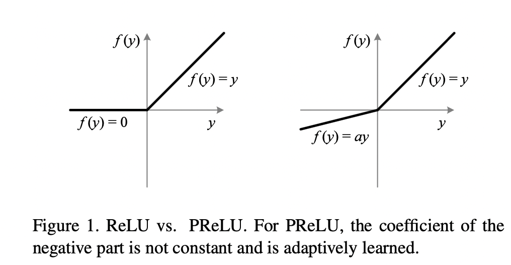
Formally, we consider an activation function defined as: \[ f(y_i)= \begin{cases} y_i, \quad & y_i > 0\\ a_i y_i, \quad & y_i \leq 0\\ \end{cases} \]
Here \(y_i\) is the input of the nonlinear activation \(f\) on the \(i\)th channel, and \(a_i\) is a coefficient controlling the slop of the negative part of the function. The subscript \(i\) in \(a_i\) indicates that we allow the nonlinear activation to vary on different channels. When \(a_i = 0\), it becomes ReLU. When \(a_i\) is small and fixed value, we have LReLU. When \(a_i\) is a learnable parameter, we call this Parametric ReLU (PReLU).
We can also rewrite the above formula as:
\[f(y_i) = \max (0, y_i) + a_i \min (0, y_i)\]
The PReLU only introduces one parameter per channel for each layer which is negligible when considering the total number of weights. At the same time, if we do not consider channels, we can use one \(a\) for all channels in same layer, the parameter number reduces to 1.
Optimization
PReLU can be trained using backpropagation and optimized simultaneously with other layers. For single layer:
\[\frac{\partial L}{\partial a_i} = \sum_{y_i} \frac{\partial L}{\partial f(y_i)} \frac{\partial f(y_i)}{\partial a_i}\]
Where \(L\) is the objective function, \(f(y_1), ...., f(y_N)\) are PReLU transformations. The gradient of PReLU transformation on single activation is given by:
\[ \frac{\partial f(y_i)}{\partial a_i} = \begin{cases} 0, \quad & y_i > 0\\ y_i, \quad & y_i \leq 0\\ \end{cases} \]
For channel shared version (single \(a\) for all channels in a layer):
\[\frac{\partial L}{\partial a} = \sum_{i} \sum_{y_i} \frac{\partial L}{\partial f(y_i)} \frac{\partial f(y_i)}{\partial a}\]
When, we can use any gradient based methods to update the parameter (e.g Momentum in this case):
\[a_i = \mu a_i + \epsilon \frac{\partial L}{\partial a_i}\]
Initialization of Filter Weights for Rectifiers
The main idea of the derivation is to investigate the variance of the response in each layer.
Forward Propagation Case
For a conv layer, a response is:
\[\mathbf{y_l} = W_{l} \mathbf{x}_l + \mathbf{b}_l\]
Where:
- \(\mathbf{x}_l\) is a \(k^2c \times 1\) vector that represents co-located \(k \times k\) pixels in \(c\) input channels (This is a joint of input pixels) and \(k\) is the kernel size (the volume after applying one kernel on the input feature maps).
- \(n = k^2c\)
- \(W_l\) is a \(d \times n\) weight matrix represents the weights in each kernel flattened in to row in \(W\).
- \(\mathbf{b}\) is a \(b \times 1\) bias vector, one dimension for each kernel.
- \(\mathbf{y}\) is the response at a pixel of the output feature map (volume \(1 \times 1 \times d\)).
- \(l\) is used to index layers.
- \(\mathbf{x}_l = f(\mathbf{y}_{l - 1})\) where \(f\) is the activation function.
- \(c_l = d_{l - 1}\) (input feature maps number is the same as kernel numbers in the previous layer).
The general idea in words is:
\(1 \times 1 \times d\) volumn of the output feature map after applying \(d\) kernels on the corresponding \(k \times k\) region of \(c\) input feature maps.
We Assume:
The initialized elements in \(W_l\) be mutually independent random variables draw from the same distribution.
The elements in \(\mathbf{x}_l\) are also mutually independent random variables draw from the same distribution.
(1) and (2) are independent.
Thus, we have:
\[Var(y_l) = Var(\mathbf{w}_l \cdot \mathbf{x}_l) = n_l Var(w_l x_l)\]
Where \(y_l, \; \mathbf{w}_l\) are rows of \(\mathbf{y}, \; W_l\) respectively, \(w_l, \; x_l\) are elements of \(\mathbf{w}_l, \; \mathbf{x}_l\)
If \(w_l\) has zero mean, then:
\[\begin{aligned} Var(y_l) &= n_l Var(w_l x_l) \\ &= n_l Var(w_l) Var(x_l) + Var(w_l)E^{2}[x_l]\\ &= n_l Var(w_l) [Var(x_l) + E^{2}[x_l]]\\ &= n_l Var(w_l) E[x^{2}_l] \end{aligned}\]Note here, in Xavier Initialization, we have \(E[x_l] = 0\) because random variables with zero means after tanh function have zero mean. For ReLU activation, we have \(x_l = max(0, y_{l - 1})\) and thus it does not have zero mean.
If we let \(w_{l - 1}\) have a symmetric distribution around zero (\(E[w_{l-1}] = 0\)) and \(b_{l - 1} = 0\), then:
\[E[y_{l - 1}] = E[w_l]E[x_l] = 0\]
Thus, \(y_{l - 1}\) has zero mean and it has a symmetric distribution around zero. This lead to:
\[\begin{aligned} E_{Y}[x^2_{l}] &= \int^{\infty}_{\infty} \max(0, y_{l - 1})^2 p_Y (y) dy\\ &= \int^{\infty}_{0} y_{l - 1}^2 p_Y (y) dy\\ &= \frac{1}{2} E[y_{l-1}^2] \end{aligned}\]Since \(\frac{1}{2} Var(y_{l - 1}) = \frac{1}{2} E[y_{l-1}^2] - \frac{1}{2} E^2[y_{l-1}] = \frac{1}{2} E[y_{l-1}^2]\):
\[\implies E_{Y}[x^2_{l}] = \frac{1}{2} Var(y_{l - 1})\]
Then, putting by this result to previous equation we have:
\[Var(y_l) = n_l Var(w_l) E[x^{2}_l] = \frac{n_l}{2} Var(y_{l - 1}) Var(w_l)\]
With \(L\) layers put together, we have:
\[\begin{aligned} Var(y_L) &= \frac{n_L}{2} Var(y_{L - 1}) Var(w_L)\\ &= \frac{n_L}{2} \frac{n_{L - 1}}{2} Var(w_L) Var(w_{L-1}) Var(y_{L - 2})\\ &= Var(y_1) \prod^{L}_{l=2} \frac{n_l}{2} Var(w_{l}) \end{aligned}\]The key is the product above, we can see that the variance of current activate depends on product of previous weights, this lead to exploding or vanishing of variance of initial activation. A proper initialization method should avoid reducing or magnifying the magnitudes of input signals exponentially.
So we expect the above product to take a proper scalar 1, a sufficient condition is:
\[\frac{1}{2} n_{l} Var(w_l) = 1, \; \forall l\]
This leads to the algorithm for forward case:
Initialize \(w_l\) from a zero-mean Gaussian distribution (\(w_l\) is assumed to be symmetric and with mean 0) whose standard deviation is \(\sqrt{\frac{2}{n_l}}\).
Initialize \(\mathbf{b} = 0\).
For the first layer, we initialize the variance to be \(\frac{1}{n_1}\).
Backward Propagation Case
For back-propagation, the gradient of a conv layer is computed by:
\[\Delta \mathbf{x}_l = [\hat{W}_l \Delta \mathbf{y}_l]_{c \times 1}\]
Where \(\frac{\partial L}{\partial \mathbf{x}} \triangleq \Delta \mathbf{x}\) and \(\frac{\partial L}{\partial \mathbf{y}} \triangleq \Delta \mathbf{y}\). Notice here, \(\Delta \mathbf{y}, \Delta \mathbf{x}\) represents the gradient for single pixel, so each of them has shape \(d_i \times 1\). Recall that, backward pass of a conv layer is also a convolution process with \(W^l\) flipped 180 degrees and applying it on gradient map of \(\mathbf{y}^l\), so \(\Delta \mathbf{y}_l\) is defined similar to \(\mathbf{x}_l\) in the forward pass. It is the \(k \times k \times d\) co-located pixels (gradients) in the output feature maps. \(\hat{W}_l\) in this case is the original kernel flipped 180 degree.
Notations:
- \(\Delta \mathbf{y}_l\) represents \(k \times k\) pixels in \(d\) dimension channels and is reshaped into a \(k^2d \times 1\) vector.
- \(\hat{n} = k^2 d\), notice here \(\hat{n} \neq n\).
- \(\hat{W}_l\) is a \(c \times \hat{n}\) matrix where the filters are rearranged in the way of back-propagation (flipped 180 degree). \(W\) and \(\hat{W}\) can be reshaped from each other.
- \(\Delta \mathbf{x}\) is a \(c \times 1\) vector representing the gradient at a pixel of the input to this layer.
Assumptions:
- We assume \(w_l\) is initialized by a symmetric distribution around zero (\(w_l, \hat{w}_l\) are from matrix but different representation so their distribution are the same).
- We assume \(w_l\), \(\Delta y_l\) are independent of each other \(\implies E[\Delta x_l] = \hat{n}_lE[w_l]E[\Delta y_l] = 0\) for all \(l\)
- We assume that \(f^{\prime} (y_l)\) and \(\Delta x_{l + 1}\) are independent.
Recall that \(\Delta \mathbf{y}_l = \Delta \mathbf{x}^T_{l + 1} \frac{\partial \mathbf{x}_{l + 1}}{\partial \mathbf{y}_l}\) and \(\frac{\partial \mathbf{x}_{l + 1}}{\partial \mathbf{y}_l}\) is a diagonal Jacobian matrix with \(f^{\prime} (y_l)\) on the diagonal, so each element of \(\mathbf{y}_l\) will have gradient \(\Delta y_l = f^{\prime} (y_l) \Delta x_{l + 1}\).
For the ReLU case, \(f^{\prime} (y_l)\) is defined as:
\[ \frac{\partial x_{l + 1}}{\partial y_l} = \begin{cases} 1, \quad & y_l \geq 0\\ 0, \quad & y_l < 0\\ \end{cases} \]
and their probabilities are equal.
Since assumption 3, we have:
\[E[\Delta y_l] = E[f^{\prime} (y_l)]E[\Delta x_{l+1}] = \frac{E[\Delta x_{l+1}]}{2} = 0\]
and also:
\[E[(\Delta y_l)^2] = Var(\Delta y_l) = Var(f^{\prime} (y_l)\Delta x_{l+1}) = \frac{Var[\Delta x_{l+1}]}{2}\]
Then the variance of gradient w.r.t to the input to layer \(l\) is:
\[\begin{aligned} Var[\Delta x_l] &= \hat{n}_l(Var(w_l)Var(\Delta y_l) + Var(w_l)E^2[\Delta y_l] + Var(\Delta y_l)E^2[w_l])\\ &= \hat{n}_lVar(w_l)Var(\Delta y_l)\\ &= \frac{\hat{n}}{2} Var(w_l) Var(\Delta x_{l + 1}) \end{aligned}\]With \(L\) layers together, we have:
\[Var(\Delta x_2) = Var(\Delta x_{L + 1}])\prod^{L}_{l=2} \frac{\hat{n}_l}{2} Var(w_l)\]
To make \(Var(\Delta x_2) = Var(\Delta x_{L + 1})\), we need to have:
\[\prod^{L}_{l=2} \frac{\hat{n}_l}{2} Var(w_l) = 1\]
Thus a sufficient condition that the gradient is not exponentially large or small:
\[\frac{\hat{n}}{2} Var(w_l) = 1\]
This results in a zero-mean Gaussian distribution whose std is \(\sqrt{\frac{2}{\hat{n}}}\)
Discussions
It is sufficient to use either forward result or backward result alone, because they only differ by a constant which is not diminishing number in common network designs. This means that if the initialization properly scales the backward signal, then this is also the case for the forward signal.
If the forward/backward signal is inappropriately scaled by a factor \(\beta\) in each layer, then the final propagated signal will be rescaled by a factor of \(\beta^L\) after \(L\) layers, where \(L\) can represent some or all layers. When \(L\) is large, if \(\beta > 1\), this leads to extremely amplified signals. If \(\beta < 1\), this leads to diminishing signal.