VGG (Under Construction)
Very Deep Convolutional Networks For Large-Scale Image Recognition
Generic Architecture
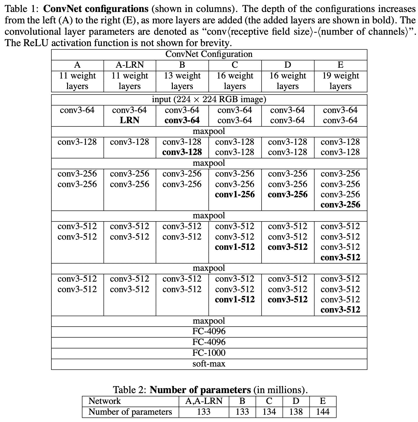
- Inputs are \(224 \times 224\) RGB images with zero mean for each pixel.
- The convolutional layers have small filter sizes (\(3 \times 3\)), one architecture with \(1 \times 1\) filters (Network C).
- Padding 1 and stride 1 to maintain the original image size.
- 5 max pooling layers with \(2 \times 2\) window and stride 2.
- 2 fully connected layers each with 4096 units, and the final fc output layer with 1000 units.
- ReLU activation function.
Configurations
the shallowest network has 11 weight layers (8 conv layers and 3 FC layers), the deepest network has 19 weight layers (16 conv layers and 3 FC layers)
The width of conv layers are relative small, starting from 64 in the first layer and then increasing by a factor of 2 each max-pooling layer, until it reaches 512.

Discussion
Instead of large filter size, we use small \(3 \times 3\) filters. We can see that after 2 consecutive layers, the effective receptive field is \(5 \times 5\), after three consective layers, the effective receptive field is \(7 \times 7\). Comparing to a conv layer with \(7 \times 7\) filter, 3 consecutive \(3 \times 3\) filter conv layers have less parameters. To see this, assume each layer has input C channel and output C channel, then total parameters:
- Single conv layer with \(7 \times 7\) filter: \(7 * 7 * C * C = 49 C^2\)
- Three conv layer each with \(3 \times 3\) filter: \(3 (3 * 3 * C * C) = 27 C^2\)
This can be seen as imposing a regularisation on the \(7 \times 7\) conv filters forcing them to have a decomposition through the \(3 \times 3\) filters. This structure also have more discriminative power (3 non-linear functions compare to one).
The \(1 \times 1\) is one way to increase the non-linearity of the decision function without affecting the receptive fields of the conv layers.
Classification Framework
Training
- Batch size 256, momentum 0.9, weight decay 0.0005
- Dropout is applied to the first two fully connected layers with rate of 0.5
Initialization
- Net \(A\) is first trained with random initialization
- When training deeper architectures, we initialize the first four conv layers and last three fully connected layers with the layer of \(A\)
- The conv layers in the middle are initialized randomly with normal(0, 0.01)
In spite of the larger number of parameters and the greater depth of our nets compare to AlexNet, the nets required less epochs to converge due to
- implicit regularization imposed by greater depth and smaller filter size
- pre-initialization of certain layers
Training Image Size Rescale
Let \(S\) (training scale) be the smallest side of an isotropically-rescaled training image from which the input image is cropped (The training input is first rescaled to smallest side = \(S\) before cropping). For a fixed crop size \(224 \times 224\), if \(S=224\), the cropped image will span the smallest side of the training image. If \(S >> 224\), the crop will correspond to a small part of the image. There are two approaches setting up \(S\)
- Single scale training: fix \(S=256, 384\)
- Multi-scale training: Each image is individually rescaled by randomly sampling \(S\) from a certain range \([S_{min}, S_{max}] = [256, 512]\).
Then the rescaled images is:
- randomly cropped from rescaled training images (one crop per image per SGD iteration)
- the crops underwent random horizontal filpping and random RGB colour shift
Testing
During Testing given a trained Conv Net and an input image:
- It is first isotropically rescaled to a predefined smallest image side \(Q\) (test scale, where \(S\) is the training scale). \(Q\) is not necessarily equal to the training scale \(S\)