Go Explore
Go-Explore: a New Approach for Hard-Exploration Problems
Definitions
What is hard-exploration problem?
- Sparse rewards: precise sequences of many actions must be taken between obtaining rewards.
- Deceptive rewards: the reward function provides misleading feedback for reaching overall global objective.
Both sparse and deceptive reward problems constitute "hard-exploration" problems.
What is Derailment?
Typical IM agents have two layers of exploration mechanisms:
- Higher level IR incentive that rewards when new states are reached, the IM agents rely on this mechanism to return to high IR promising states.
- A more basic exploratory mechanism such as epsilon-greedy exploration, action-space noise, or parameter-space noise. The IM agents rely on this mechanism to explore high IR states.
However, to return to a previously discovered high IR state, a longer, more complex and more precise sequence of actions is needed. In this case, the lower level exploration mechanism (e.g epsilon greedy) will "derail" the agent from ever returning to that state (The needed precise actions are naively perturbed by the basic exploration mechanism).
What is detachment?
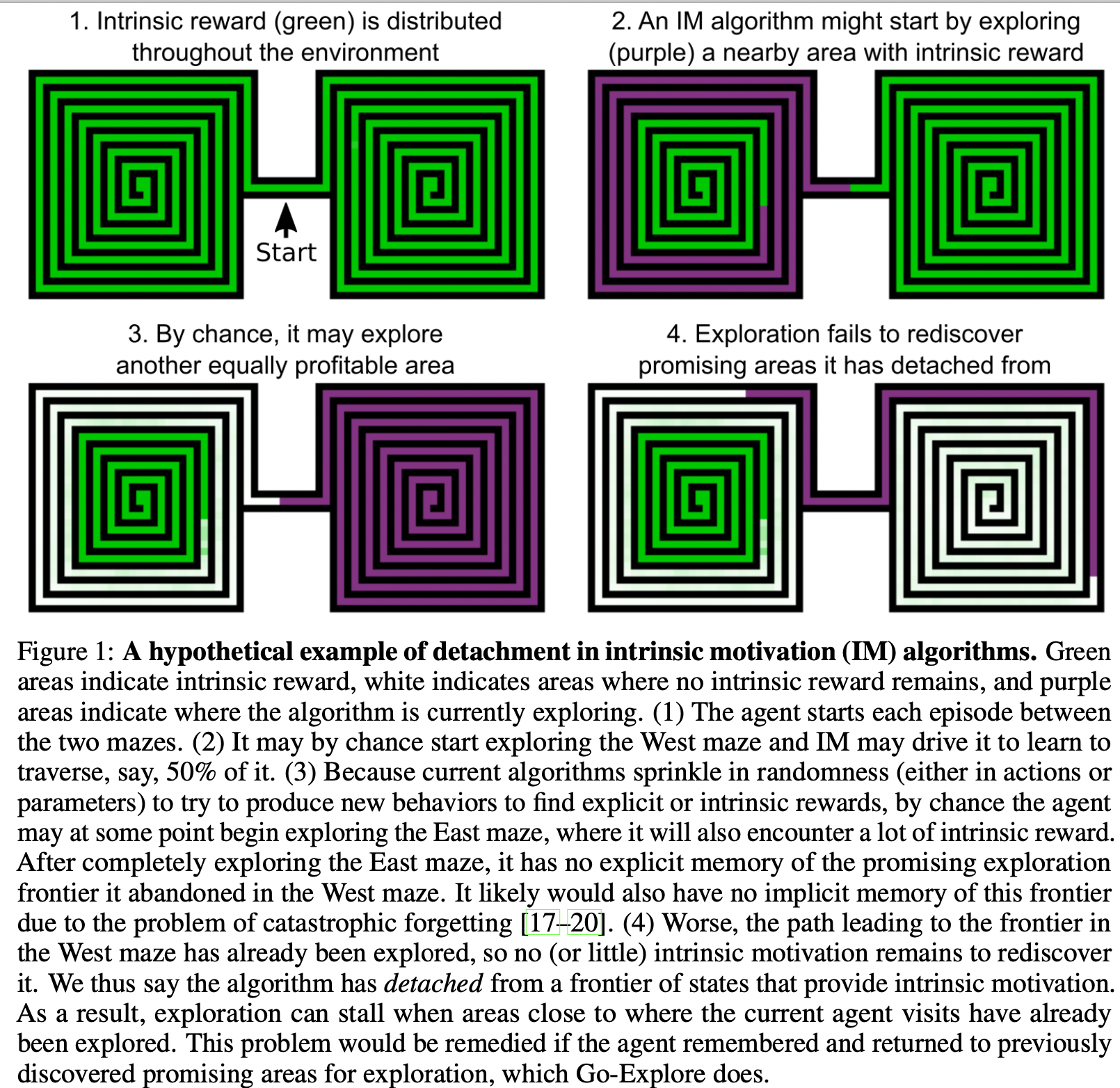
Detachment is idea that an agent driven by Intrinsic Motivation could become detached from the frontiers of high intrinsic reward. IM is nearly always a consumable resource: a curious agent is curious about state to the extent that it has not often visited them. If an agent discovers multiple areas of the state space that produce high IR, its policy may in the short term focus on one such area. After exhausting some of the IR offered by that area, the policy may by chance begin consuming IR in another area. Once it has exhausted that IR, it is difficult for it to rediscover the frontier it detached from in the initial area, because it has already consumed the IR that led to that frontier and it likely will not remember how to return to that frontier due to catastrophic forgetting.
In theory, a replay buffer could prevent detachment, but in practicce it would have to be large to prevent data about the abandoned frontier to not be purged before it becomes needed, and large replay buffers introduce their own optimization stability difficulties.
Go Explore Algorithm
Go-Explore is an explicit response to both detachment and derailment that is also designed to achieve robust solutions in stochastic environments. To deal with:
- Detachment: The algorithm explicitly stores an archive of promising states visited so taht they can then be revisited and explored from later.
- Derailment: The algorithm decomposes the basic exploration mechanism into first returning to a promising state without intentionally adding any exploration then exploring further from the promising state.
The algorithm works in two phases:
Phase 1: solve the problem in a way that may be brittle, such as solving a deterministic version of the problem. Phase 1 focuses on exploring infrequently visited states which forms the basis for dealing with sparse-reward and deceptive problems.
- Add all interestingly different states visited so far into the archive
- Each time a state from the archive is selected to explore from, first GO back to the state without adding exploration, and then Explore further from that state in search of new states.
Phase 2: robustify (train to be able to reliably perform the solution in the presence of stochasticity) via imitation learning or learning from demonstrations. The only difference with Go-Explore is that the solution demonstrations are produced automatically by Phase 1 instead of being provided by humans. If in the first phase, we obtain a policy that is robust in stochastic environment, then we do not need this second phase.
- Input: One or more high-performing trajectories from phase 1
- Output: A robust policy able to consistently achieve similar performance.
Phase 1: Explore until solved
The purpose of Phase 1 is to explore the state space and find one or model high-performing trajectories that can later be turned into a robust policy in Phase 2. To do this, phase 1 builds up an archive of interestingly different game states, which we call cells, and the trajectories that lead to them. It starts with an archive that only contains the starting state. From there, it builds the archive by repeating the following procedure:
choose a cell from the current archive
return to that cell without adding any stochastic exploration
explore from that location stochastically
Cell representations
In theory, one can store high-dimensional states as cell with one cell representing one state. However, this is intractable in practice. To be tractable in high-dimensional state spaces, we need to reduce the dimensionality of the state space (although the final policy will still play in the same original state space). Thus, we want the cell representation to conflate similar states while not conflating states that are meaningfully different (aggregating similar frames to one frame).
Since appropriate downscaling parameters can vary across games and even as exploration progresses within a given game, such parameters are optimized dynamically at regular intervals by maximizing the objective function over a sample of recently discovered frames.
Cell representations without domain knowledge
We found that a very simple dimensionality reduction procedure produces surprisingly good results on Montezuma's Revenge. Specifically:
- Convert each game frame image to grayscale
- Downscale it to an \(w \leq 160, \; h \leq 120\) image with area interpolation (i.e using the average pixel value in the area of the downsampled pixel)
- rescale pixel intensities \(d \leq 255\) using the formula \(\lfloor \frac{d\cdot p}{255} \rfloor\), instead of original 0 to 255.
The downscaling dimensions and pixel-intensity range \(w, h, d\) are updated dynamically by proposing different values for each, calculating how a sample of recent frames would be grouped into cells under these proposed parameters, and then selecting the values that result in the best cell distribution as determined by the objective function:
The objective function for candidate downscaling parameters is calculated based on:
A target number of cells \(T\), where \(T\) is a fixed fraction of the number of cells in the sample (target groups of frames formed from the samples of frames)
The actual number of cells produced by the parameters currently considered, \(n\) (actual groups of frames formed from the samples)
The distribution of sample frames over cells \(\mathbf{p}\)
\[O(\mathbf{p}, n) = \frac{H_n (\mathbf{p})}{L(n, T)}\]
Where:
Cell number control: \(L(n, T)\) measures the discrepancy between the number of cells under the current parameters \(n\) and the target number of cells \(T\). It prevents the representation that is discovered from aggregating too many frames together, which would result in low exploration, or from aggregating too few frames together, which would result in an intractable time and memory complexity.
\[L(n, T) = \sqrt{|\frac{n}{T} - 1| + 1}\]
If \(n >> T \implies L(n, T) \rightarrow \infty\), if \(n << T \implies L(n, T) \rightarrow \sqrt{2}\), more penalty on large number of groups.
Frame distribution control: \(H_n (\mathbf{p})\) is the ratio of the entropy of how frames were distributed across cells to the entropy of the discrete uniform distribution of size \(n\).
\[H_n (\mathbf{p}) = - \sum^{n}_{i=1} \frac{p_i \log(p_i)}{\log(n)}\]
Larger entropy gives a uniform distribution, that is, the objective encourages frames to be distributed as uniformly as possible across cells. Normalized entropy is comparable across different number of cells, allowing the number of cells to be controlled solely by \(L(n, T)\).
At each step of the randomized search, new values of each tuple of parameter \(w, h, d\) are proposed by sampling from a geometric distribution (close to zero values have higher probability of being selected) whose mean (\(\mu = \frac{1}{p}\)) is the current best known value of the given parameter. If the current best known value is lower than a heuristic minimum mean \(w=8, h=10.5, d=12\), then the minimum mean is used as the mean of the geometric distribution. New parameter values are resampled if they fall outside of the valid range for the parameter. Then, the scaled frames are grouped into groups and objective are calculated.
The sample of frames are obtained by maintaining a set of recently seen smaple frames as GO-Explore runs: each time a frame not realy in the set is seen during the explore step, it is added to the running set with a probability of 1%. If the resulting set contains more than 10,000 frames, the oldest frame it contains is removed.
Cell representations with domain knowledge
In Montezuma's Revenge, domain knowledge is provided as unique combinations of:
the \(x, y\) position of the agent (descretized into a grid in which each cell is \(16 \times 16\) pixels)
room number
level number
rooms that the currently-held keys were found
In Pitfall, only the \(x, y\) position of the agent and room number is used.
All of this information was extracted directly from pixels with simple hand-coded classifiers to detect objects such as the main character's location combined with our knowledge of the map structure in the two games.
While Phase 1 provides the opportunity to leverage domain knowledge in the cell representation, the robustified Neural Network produced by Phase 2 still plays directly form pixels only.
Selecting cells
In each iteration of Phase 1, a cell is chosen from the archive to explore from. This choice could be made:
- Uniformly at random
- Assign a positive weight to each cell that is higher for cells that are deemed more promising (less often visited cells, have recently contributed to discovering a new cell, expected to be near undiscovered cells and etc..). The weights of all cells are normalized to represent the probability distribution over the current cell space. No cell is ever given a weight of 0.
Count Subscore
The score of a cell is the sum of separate subscores. One important set of such subscores is called the count subscores. Count subscores are computed from attributes of cells that represent the number of times a cell was interacted with in different ways. Specifically:
The number of times the cell has already been chosen (i.e selected as a cell to explore from)
The number of times the cell was visited at any point during the exploration phase
the number of times a cell has been chosen since exploration from it last produced the discovery of a new or better cell.
Lower counts of these attributes indicate a more promising cell to explore from (e.g. a cell that has been chosen more times already is less likely to lead to new cells than a cell that has been chosen fewer times). The count subscore for each of these attribute is given by:
\[CntScore (c, a) = w_a \cdot (\frac{1}{v(c, a) + \epsilon_1})^{p_a} + \epsilon_2\]
Here:
\(c\) is the cell for which we are calculating the score
\(v(c, a)\) is the value of attribute \(a\) for cell \(c\)
\(w_a\) is the weight hyperparameter for attribute \(a\)
\(p_a\) is the power hyperparameter for attribute \(a\)
\(\epsilon_1\) is a normalization parameter to prevent zero division
\(\epsilon_2\) helps guarantee that no cell ever has a 0 probability of being chosen
\(\epsilon_1=0.001, \epsilon_2=0.00001\) are the default values.
Neighbor Subscore
Given the position of \(x, y\), it is possible to determine the possible neighbors of given cells and whether these neighbors are already present in the archive. For these cases, we define a set of neighbor subscores. Each neighbor subscore is defined as \(w_n\) if neighbor \(n\) does not exist in the archive, 0 if the does exist.
The motivation of neighbor subscore is that the cells that are lacking neighbors are likely at the edge of the current frontier of knowledge and are thus more likely to yield new cells. We consider 3 types of neighbors:
- Vertical (2)
- Horizontal (2)
- Cells that are in the same level, room, \(x, y\) position, but are holding a larger number of keys
Neighbors of the same type share the same value for \(w_n\), then the score is calculated by:
\[NeighScore(c, n) = w_n * (1 - HasNeighbor(c, n))\]
Where \(c\) is current cell and \(n \in Vertical \cup Horizontal \cup MoreKeys\) is current neighbor. In cases without domain knowledge, it is unclear what exactly would constitute a cell's neighbor, and so neighbor score is defined as 0.
Level Weight (Only Montezuma's Revenge)
In the case of Montezuma's Revenge with domain knowledge, cells are exponentially downweighted based on the distance to the maximum level currently reached, thereby favoring progress in the furthest level reached, while skill keeping open the possibility of improving previous level's trajectories:
\[LevelWeight (c) = 0.1^{MaxLevel - Level(c)}\]
In the case of no domain knowledge, \(LevelWeight (c) = 1, \quad \forall c\)
Final Score and Final Cell Probability
The final score is then:
\[CellScore (c) = LevelWeight (c) \cdot [(\sum_n NeighScore (c, n)) + \sum_a CntScore (c, a) + 1]\]
The final probability is then:
\[CellProb (c) = \frac{CellScore (c)}{\sum_{c^{\prime}}CellScore (c^{\prime})}\]
New Version
In the new version (except Montezuma's Revenge with domain knowledge but without a return policy), the selection weight (score) is reduced to:
\[W = \frac{1}{\sqrt{C_{seen} + 1}}\]
In case of Montezuma's Revenge with domain knowledge but without a return policy, three addtional domain knowledge features further contribute to the weight:
The number of horizontal neighbours to the cell present in the archive (\(h\)).
A key bonus: for each location (defined by level, room, and x, y position), the cell with the largest number of keys at that location gets a bonus of \(k=1\) (\(k=0\) for other cells).
The current level.
\[W_{location} = \frac{2 - h}{10} + k\] \[W_{mont_domain} = 0.1^{L-l}(W + W_{location})\]
Where, \(l\) is the level given current cell and the maximum level in the archive \(L\).
Returning to cells and opportunities to exploit deterministic simulators
The easiest way to return to a cell is if the world is deterministic and resettable, such that one can reset the state of the simulator to a previous visit to that cell. The ability to harness determinism and perform such resets forces us to recognize that there are two different types of problems we wish to solve with RL algorithms:
- Require stochasticity at test time only
- Require stochasticity during both testing and training time (further research)
- Environment that prevents return to cells (further research)
We can take advantage of the fact simulators can be made deterministic to improve performance, especially on hard-exploration problems. For many types of problems, we want a reliable final solution (e.g. a robot that reliably finds survivors after a natural disaster) and there is no principled reason to care whether we obtain this solution via initially deterministic training. If we can solve previously unsolvable problems, including ones that are stochastic at evaluation (test) time, via making simulators deterministic, we should take advantage of this opportunity.
There are also cases where a simulator is not available and where learning algorithms must confront stochasticity during training. We can train goal-conditioned policies that reliably return to cells in the archive during the exploration phase. This strategy would result in a fully trained policy at the end of the exploration phase meaning there would be no need for a phase 2 at the end.
For problems in which all we care about is a reliable policy at test time, a key insight behind Go-Explore is that we can first solve the problem (Phase 1), and then (if necessary) deal with making the solution more robust later (Phase 2).
Due to the fact that the present version of Go-Explore operates in a deterministic setting during Phase 1, each cell is associated with an open-loop sequence of instructions that lead to it given the initial state, not a proper policy that maps any state to an action. A true policy is produced during robustification in Phase 2.
Sequence of actions and states are stored for each cell
Exploration from cells
Once a cell is reached, any exploration method can be applied to find new cells. In this work, the agent explores by taking random actions \(k = 100\) training frames, with a 95% probability of repeating the previous action at each training frame. Besides reaching the \(k = 100\) training frame limit for exploration, exploration is also aborted at the episodes' end, and the action that led to the episode ending is ignored because it does not produce a destination cell.
This exploration does not require a neural network or other controller.
Updating the archive
While an agent is exploring from a cell, the archive updates in two conditions:
When the agent visits a cell that was no yet in the archive (which can happen multiple times while exploring from a given cell). In this case, , that cell is added to the archive with four associated pieces of meta data:
- A full trajectory from the starting state to that cell (states and actions)
- The state of the environment at the time of discovering the cell (if the environment supports such an operation)
- The cumulative score of that trajectory
- The length of that trajectory
The second condition is when a newly-encountered trajectory is "better" than that belonging to a cell already in the archive. We define a new trajectory is "better" than an existing trajectory when the new trajectory either has:
- A higher cumulative score
- A shorter trajectory with the same score
In either case, we update the existing cell in the archive with new trajectory, new trajectory length, new environment state and new score. In addition, information regarding the likelihood of this cell being chosen resets including the total number of times the cell has been chosen and the number of times the cell has been chosen since leading to the discovery of another cell. Resetting these values is beneficial when cells conflate many different states because a new way of reaching a cell may actually be a more promising stepping stone to explore from (so we want to encourage its selection).
Batch Implementation
Phase 1 is implemented in parallel to take advantage of multiple CPUs. At each step, a batch of \(b\) cells is selected with replacement and exploration from each of these cells proceeds in parallel. A high \(b\) saves time of recomputing cell selection probabilities less frequently, which is important as this computation accounts for a significant portion of run time as the archive gets large.
Phase 2
If successful, the result of Phase 1 is one or more high-performing trajectories. However, if Phase 1 of Go-Explore harness ed determinism in a simulator, such trajectories will not be robust to any stochasticity, which is present at test time. Phase 2 addresses this gap by creating a policy robust to noise via imitation learning. Thus, the policy that is trained has to lean how to mimic or perform as well as the trajectory obtained from the Go-Explore exploration phase while simultaneously dealing with circumstances that were not present in the original trajectory.
The Backward Algorithm is used for imitation learning. It works by starting the agent near the last state in the trajectory, and then running an ordinary RL algorithm from there (In this case PPO). Once the algorithm has learned to obtain the same or a higher reward than the example trajectory from that starting place near the end of the trajectory, the algorithm backs the agent's starting point up to a slightly earlier place along the trajectory and repeats the process until eventually the agent has learned to obtain a score greater than or equal to the example trajectory all the way from the initial state.
Advantages:
- The policy is only optimized to maximize its own score, and not actually forced to accurately mimic the trajectory, for this reason, this phase is able to further optimize the expert trajectories as well as generalize beyond them.
- RL algorithms with discounting factor that prizes near-term rewards more than those gathered later. Thus, if the original trajectory contains unnecessary actions, such behavior could be eliminated during robustification.
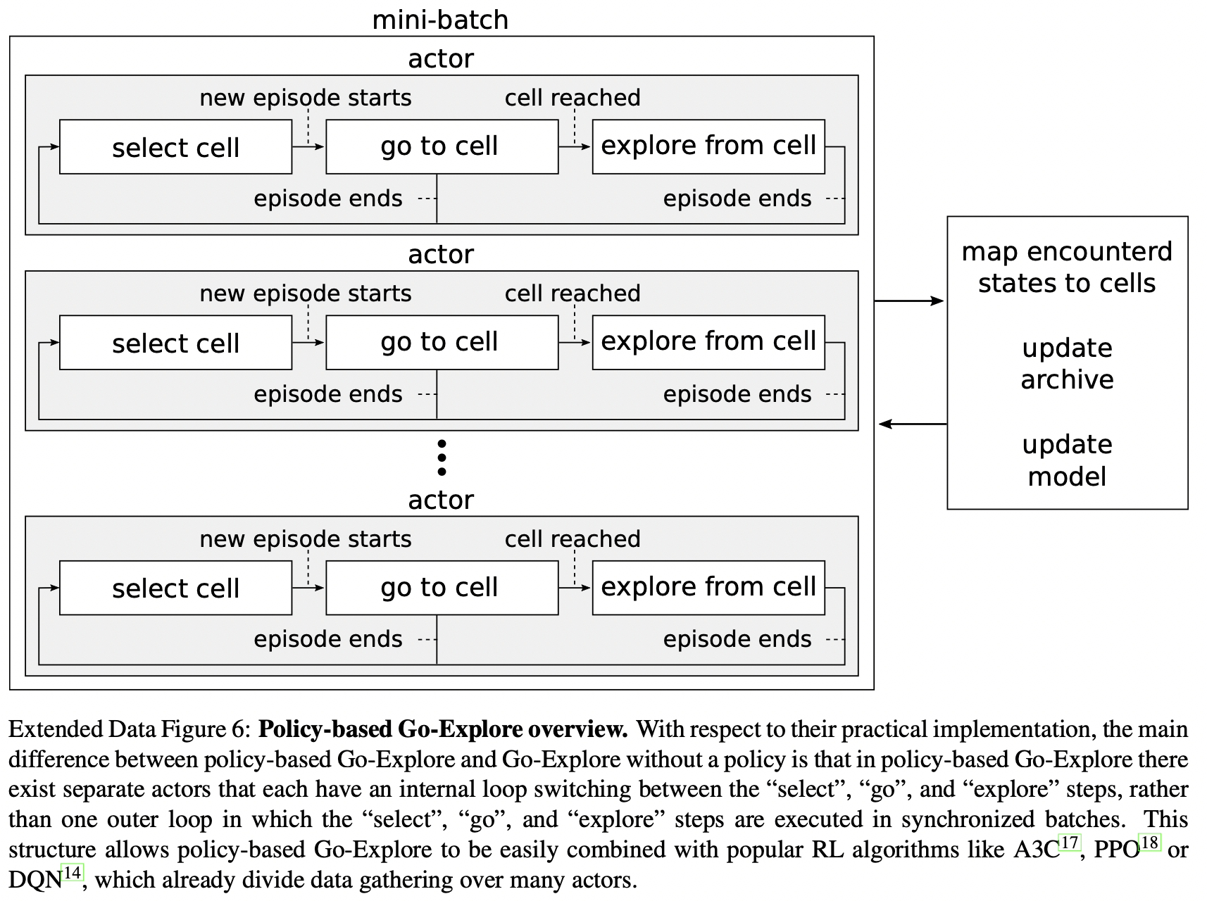
Policy-based Go-Explore
In policy-based Go-Explore, a goal-conditioned (i.e conditioned on the cell to return to) policy \(\pi_{\theta} (a | s, g)\) is trained during the exploration phase with PPO. Instead of training the policy to directly reach cells in the archive, the policy is trained to follow the best trajectory of cells that previously led to the selected state (cell). The goal-conditioned policy has the potential to greatly improve exploration effectiveness over random actions. In addition to returning to previously visited cells, the policy can also be queried during the explore step by presenting it with additional goals, including goals not already in the archive. Such goal cells are chosen according to a simple strategy that either:
Chooses a cell adjacent to the current position of the agent, possibly leading to a new cell.
Randomly selects a cell from the archive, potentially repositioning the agent within the archive or finding new cells while trying to do so.
Every time post-return exploration (after reaching the selected cell from archive) is started, the algorithm randomly commits with equal probability to either take random actions or sampling from the policy for the duration of the post-return exploration step.
The total reward \(r_t\) is the sum of the trajectory reward \(r^{\tau}_t\) and the environment reward \(r^e_t\), where \(r^e_t\) is clipped to the \([-2, 2]\) range. Policy based Go-Explore also includes self-imitation learning, where self-initation actors follow the same procedure as regular actors, except that they replay the trajectory associated with the cell they select from the archive.