Xavier Initialization

Understanding the Difficulty of Training Deep Feedforward Neural Networks

The analysis is driven by investigative experiments to monitor activations (watching for saturation of hidden units) and gradients, across layers and across training iterations.

Experimental Setting

Feedforward neural networks with one to five hidden layers, one thousand hidden units per layer and a softmax logistic regression for the output layer are optimized. The cost function is the negative log-liklihood \(-\log p_{Y | X}(y | x)\), where \((x, y)\) is the (input image, target class) ordered pair. The neural networks were optimized with stochastic back-propagation on mini-batches of size ten. An average gradient over the mini-batch are used to update parameters \(\theta\) in that direction, with \(\theta \leftarrow \theta - \epsilon g\).

We varied the type of non-linear activation function in the hidden layers:

1. Sigmoid: \(\frac{1}{(1 + e^{-x})}\)
2. Hyperbolic tangent: \(tanh (x)\)
3. Softsign: \(\frac{x}{(1 + |x|)}\) (similar to tanh but approaches asymptotes much slower, softer slope)

The initial weights \(W_{i, j} \sim U[-\frac{1}{\sqrt{n}}, \frac{1}{\sqrt{n}}]\), biases are initialized to 0. Where \(n\) is the size of the previous layer.

Effect of Activation Functions and Saturation During Training

Experiments with the Sigmoid

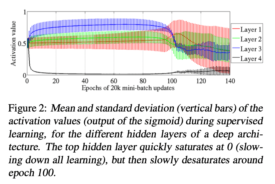
The graph shows the mean and standard deviation of activations after apply sigmoid function for each layer(activations are computed using a fixed set of 300 test examples at different time during training). We can see very clearly that the deepest layer (top layer) at the beginning have all activation values around lower saturation value of 0. Inversely, the others layers have a mean activation value that is above 0.5 and decreasing as we go from the output layer to the input layer.

With random initialization, the lower layers of the network computes initially is not useful to the classification task, so the output layer \(softmax(b + Wh)\) might initially rely more on the bias \(b\) (which are learned very quickly) than on the top hidden activations \(h\) derived from the input image (because \(h\) may not be predictive at beginning due to random initialization). Thus, the error gradient would tend to push \(Wh\) towards 0, which can be achieved by pushing \(h\) towards 0 (saturation regime of the sigmoid activation function). Then, this will prevent gradients to flow backward and prevent the lower layers form learning useful features. Eventually but slowly, the lower layers move toward more useful features and the top hidden layer then moves out of the saturation regime.

Experiments with the Tanh and Softsign

The hyperbolic tangent networks do not suffer from the kind of saturation behavior of the top hidden layer observed with sigmoid network (tanh (0) has large gradient norm). However, sequentially saturation can occur starting with layer 1 and propagating up in the network (one by one).

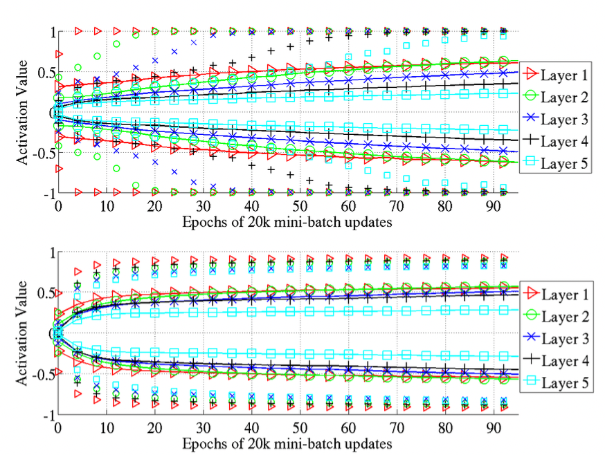
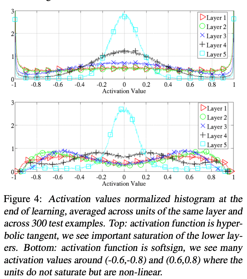
The softsign is similar to tanh but behave differently in terms of saturation because of its smoother asymptotes. We can see that the saturation does not occur one layer after the other like for the tanh, it is faster at the beginning and then slow, and all layers move together towards larger weights.

Studying Gradients and their Propagation

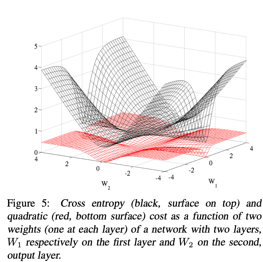
Effect of the Cost Function

The loss function is very important in terms of better learning. In classification, cross entropy (negative log-likelihood) couped with softmax outputs worked much better than quadratic cost. The plateaus in the traning criterion are less present with the log-likelihood cost-function.

Gradients at Initialization

We will start by studying the linear regime (activation). For a dense artificial NN using symmetric activation function \(f\) with unit derivative at 0 (ie. \(f^{\prime} (0) = 1\)). If we write \(\mathbf{z}^{i}\) for the activation vector of layer \(i\) (row vector), and \(\mathbf{s}^i\) the argument vector of the activation function at layer \(i\), we have (denominator layout):

\[\mathbf{s}^{i}_{1 \times d} = \mathbf{z}^{i} W^i + \mathbf{b}^{i}\]

and \(\mathbf{z}^{i+1} = f(\mathbf{s}^{i})\), Then:

\[\begin{aligned} {\frac{\partial Cost}{\partial s^{i}_{k}}}_{1 \times 1} &= \frac{\partial \mathbf{z}^{i + 1}}{\partial s^{i}_{k}}\frac{\partial \mathbf{s}^{i+1}}{\partial \mathbf{z}^{i + 1}}\frac{\partial Cost}{\partial \mathbf{s}^{i+1}}\\ &= [\frac{\partial z^{i + 1}_1}{\partial s^{i}_{k}} ... \frac{\partial z^{i + 1}_k}{\partial s^{i}_{k}} ... \frac{\partial z^{i + 1}_d}{\partial s^{i}_{k}}] W^{i} \frac{\partial Cost}{\partial \mathbf{s}^{i+1}}\\ &= [0 ... f^{\prime} (s^{i}_{k}) ... 0] W^{i + 1} \frac{\partial Cost}{\partial \mathbf{s}^{i+1}}\\ &= [f^{\prime} (s^{i}_{k}) W^{i + 1}_{k, \cdot}]_{1 \times d} \frac{\partial Cost}{\partial \mathbf{s}^{i+1}}_{d \times 1}\\ \\ \frac{\partial Cost}{\partial w^{i}_{l, k}}_{1 \times 1} &= \frac{\partial \mathbf{s}^{i}}{\partial w^{i}_{l, k}}_{1 \times d} \frac{\partial Cost}{\partial \mathbf{s}^{i}}_{d \times 1}\\ &= [0 ... \frac{\partial s^{i}_{k}}{\partial w^{i}_{l, k}} ... 0] \frac{\partial Cost}{\partial \mathbf{s}^{i}}\\ &= z^{i}_{l} \frac{\partial Cost}{\partial s^{i}_{k}}\\ \end{aligned}\]

Assume that we are in a linear regime (activation) at the initialization, that the weights are initialized i.i.d with mean zero , same variance (i.e \(Var[w^{l}_1] = Var[w^l_i] = Var[w^l]\)) and that the inputs features have mean zero and variances are the same (i.e \(Var[x_1] = Var[x_i] = Var[x]\)), we can say that with \(n_i\) the size of layer \(i\) and \(\mathbf{x}\) the network input:

\[f^{\prime} (s^i_k) \approx 1\]

\[Var[\mathbf{z}^{1}] = Var[\mathbf{x}W^{0} + \mathbf{b}^{0}] = n_{0}[Var[x]Var[w^{0}]]_{1 \times d} = n_0 Var[\mathbf{x}] Var[W^0]\]

\[Var[\mathbf{z}^{i}] = Var[\mathbf{z^{i - 1}}W^{i - 1} + \mathbf{b}^{i - 1}] = Var[\mathbf{x}] \prod^{i - 1}_{i^{\prime} = 0} n_{i^{\prime}}Var[W]^{i^{\prime}}\]

Where \(Var[W^{l}] = [Var[w^l]]_{n_{l - 1} \times n_{l}}\) is the shared scalar variance of all weights at layer \(l\). Then for a network with \(d\) layers:

\[\begin{aligned} Var[\frac{\partial Cost}{\partial \mathbf{s}^{i}}] &= Var[\frac{\partial \mathbf{z}^{i + 1}}{\partial \mathbf{s}^{i}} W^{i + 1} \frac{\partial Cost}{\partial \mathbf{s}^{i+1}}]\\ &= Var[W^{i + 1} \frac{\partial Cost}{\partial \mathbf{s}^{i+1}}]\\ &= Var[W^{i + 1}W^{i + 2}\frac{\partial Cost}{\partial \mathbf{s}^{i+2}}]\\ &= (\prod^{d}_{i^{\prime} = i} n_{i^{\prime} + 1} Var[W^{i^{\prime}}]) Var[\frac{\partial Cost}{\partial \mathbf{s}^{d}}] \\ \\ \\ Var[\frac{\partial Cost}{\partial w^{i}_{l, k}}] &= Var[z^{i}_{l} \frac{\partial Cost}{\partial s^{i}_{k}}]\\ &= Var[x] \prod^{i - 1}_{i^{\prime} = 0} n_{i^{\prime}} Var[w^{i^{\prime}}] \prod^{d}_{i^{\prime} = i} n_{i^{\prime} + 1} Var[w^{i^{\prime}}]\\ &= \prod^{i - 1}_{i^{\prime} = 0} n_{i^{\prime}} Var[w^{i^{\prime}}] \prod^{d}_{i^{\prime} = i} n_{i^{\prime} + 1} Var[w^{i^{\prime}}] \times Var[x] Var[\frac{\partial Cost}{\partial s^{d}}] \end{aligned}\]

From a forward-propagation point of view (We want to make sure that we have similar variance initialization at deeper layers as all layers, so we do not stuck at small gradients at beginning), we would like to keep things flowing (want inputs to have similar mean and variance, similar distribution):

\[Var[z^{i}] = Var[z^{i^{\prime}}]\]

This transforms to:

\[Var[x] \prod^{i - 1}_{k = 0} n_{k} Var[w^{k}] = Var[x] \prod^{i^{\prime} - 1}_{j = 0} n_{j} Var[w^{j}]\]

\[\implies \prod^{\max (i - 1, i^{\prime} - 1)}_{j = \max (i - 1, i^{\prime} - 1) - \min (i - 1, i^{\prime} - 1)} n_j Var(w^j) = 1 \]

If we let \(Var[w^i] = \frac{1}{n_i}\), then the above condition is satisfied for \((i, i^{\prime})\).

From a back-propagation point of view (We want to have similar variance so no gradients exploding or vanishing at the beginning), we would similarly like to have the gradients to have similar variance as we backpropagate through layers:

\[Var[\frac{\partial Cost}{\partial s^{i^{\prime}}}] = Var[\frac{\partial Cost}{\partial s^{i}}]\]

\[\implies (\prod^{d}_{j = i^{\prime}} n_{j + 1} Var[w^{j}]) Var[\frac{\partial Cost}{\partial s^{d}}] = (\prod^{d}_{k = i} n_{k + 1} Var[w^{k}]) Var[\frac{\partial Cost}{\partial s^{d}}]\]

\[\implies \prod^{\max (i - 1, i^{\prime} - 1)}_{j = \min (i - 1, i^{\prime} - 1)} n_{j + 1} Var(w^j) = 1\]

If we let \(Var[w^i] = \frac{1}{n_{i + 1}}\), then the above condition is satisfied for \((i, i^{\prime})\).

Thus, we have two conditions (to ensure no gradient exploding and vanishing):

\[Var[w^i] = \frac{1}{n_{i + 1}} \quad \quad Var[w^i] = \frac{1}{n_i}\]

When all layers have same size, we can satisfy both conditions. However, in most cases, we do not have this condition satisfied. Thus, by combining and compromising, we have:

\[Var[w^i] = \frac{2}{n_{i} + n_{i + 1}}\]

This initialization is called normalized initialization.

Example:

If we have initialization \(w^{i} \sim U[-\frac{1}{\sqrt{n_{i - 1}}}, \frac{1}{\sqrt{n_{i - 1}}}]\), then the variance is \(Var[w^{i}] = \frac{1}{3 n_{i - 1}}\). This will cause the variance to depend on the layer and decreasing. The normalization factor may therefore be important when initializing deep networks because of the multiplicative effect through layers. Thus, we can refine this to be: \[w^{i} \sim U[-\frac{\sqrt{6}}{\sqrt{n_{i + 1} + n_{i}}}, \frac{\sqrt{6}}{\sqrt{n_{i + 1} + n_{i}}}]\] then the variance \(Var[w^{i}] = \frac{2}{n_{i} + n_{i + 1}}\)

Back-propagated Gradients During Learning

The dynamic of learning in NN is complex and we would like to develop better tools to analyze and track it. In particular, we cannot use simple variance calculations like above because the weights values are not anymore independent of the activation values and the linearity hypothesis is also violated.

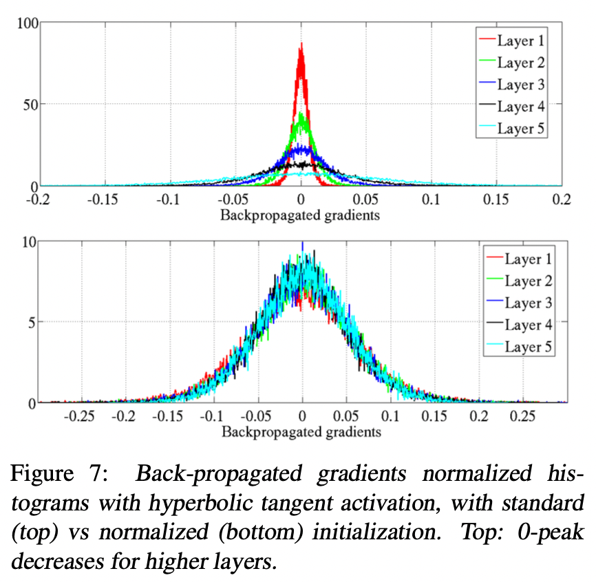
From the above graph, we can see that at the beginning of training:

1. The gradient variance gets smaller as it is propagated downwards.
2. The distribution of gradient is roughly the same using normalized initialization.

Conclusions

1. The more classical NN with sigmoid or hyperbolic tangent units and standard initialization fare rather poorly, converging more slowly and apparently towards ultimately poorer local minima.
2. The softsign networks seem to be more robust to the initialization procedure than the tanh network.
3. For tanh networks, the proposed normalized initialization can be quite helpful, because the layer to layer transformation maintain magnitudes of activations and gradients.
4. Sigmoid activations should be avoided when initializing from small random weights, because they yield poor learning dynamics with initial saturation of the top hidden layer.
5. Keeping the layer to layer transformations such that both activations and gradients flow well (i.e with a jacobian around 1) appears helpful.