Calculus (2)

Multivariate Calculus (2)

Double Integrals

Double Integrals over Rectangles

In a similar manner as definite integral, we consider a function \(f\) of two variables defined on a closed rectangle:

\[R = [a, b] \times [c, d] = \{(x, y, z) \in \mathbb{R}^2 | a \leq x \leq b, c \leq y \leq d\}\]

and we first suppose that \(f(x, y) \leq 0\). The graph of \(f\) is a surface with equation \(z = f(x, y)\). Let \(S\) be the solid that lies above \(R\) and under the graph of \(f\):

\[S = \{(x, y, z) \in \mathbb{R}^3 | a \leq x \leq b, c \leq y \leq d, 0 \leq z \leq f(x, y)\}\]

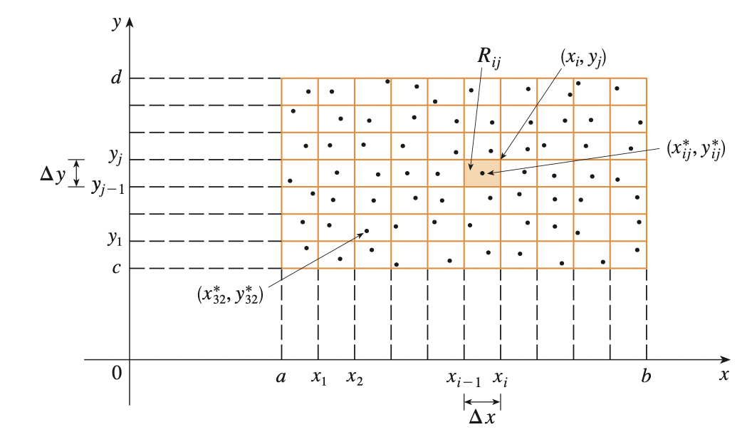
We first divide the \(R\) into subrectangles. We accomplish this by dividing the interval \([a, b]\) into \(m\) subintervals \([x_{i-1}, x_{i}]\) of equal width \(\Delta x = \frac{(b - a)}{m}\) and dividing \([c, d]\) into \(n\) subintervals \([y_{j - 1}, y_j]\) of equal width \(\Delta y = \frac{(d - c)}{n}\). Then the subrectangles are defined as:

\[R_{i, j} = [x_{i - 1}, x_i] \times [y_{j - 1}, y_j] = \{(x, y) | x_{i - 1} \leq x \leq x_i, y_{j - 1} \leq y leq y_j\}\]

Then the area of individual subrectangle is:

\[\Delta A = \Delta x \Delta y\]

If we choose a sample point \((x^{*}_{i, j}, y^{*}_{i, j}) \in R_{i, j}\), then we can approximate the part of \(S\) that lies above each \(R_{i, j}\) (The volume) by a column with height \(f(x^{*}_{i, j}, y^{*}_{i, j})\) and base area \(\Delta A\). The volume of the column:

\[f(x^{*}_{i, j}, y^{*}_{i, j})\Delta A\]

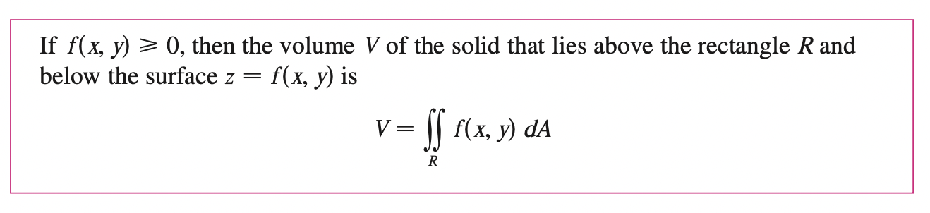
Then the volume (only when \(f(x, y) \leq 0 \; \forall (x, y) \in S\)) of \(S\) can be approximated:

\[V \approx \sum^{m}_{i=1} \sum^{n}_{j=1}f(x^{*}_{i, j}, y^{*}_{i, j})\Delta A\]

This sum is called double Riemann sum.

Then the approximation becomes better as \(n, m \rightarrow \infty\):

\[V = \lim_{n, m \rightarrow \infty} \sum^{m}_{i=1} \sum^{n}_{j=1}f(x^{*}_{i, j}, y^{*}_{i, j})\Delta A\]

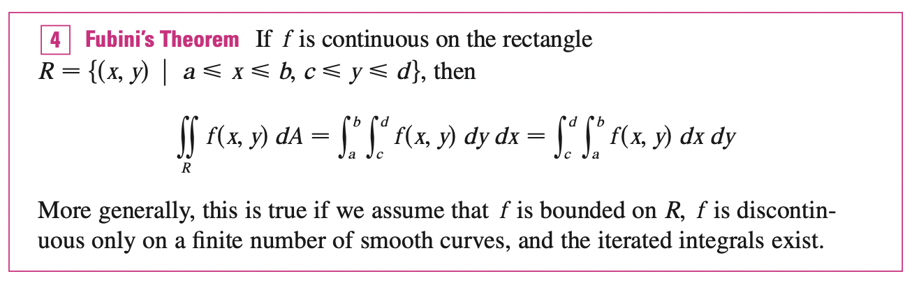
A function \(f\) is called integrable if the limit above exists, it can be showed that all continuous functions are integrable. If \(f\) is bounded (\(\exists \; M, \; s.t \; |f(x, y)| \leq M, \; \forall (x, y) \in R\)), then if \(f\) is continuous there, except on a finite number of smooth curves, then \(f\) is integrable over \(R\).

Iterated Integral

Suppose that \(f\) is a function of two variables that is integrable on the rectangle \(R = [a, b] \times [c, d]\). Now, \(\int^{d}_{c} f(x, y) dy\) is a function that depends on the value of \(x\):

\[A(x) = \int^{d}_{c} f(x, y) dy\]

If we now integrate the function \(A\) w.r.t \(x\) from \(a\) to \(b\), we have:

\[\int^{b}_{a} A(x) dx = \int^{b}_{a} \int^{d}_{c} f(x, y) dy dx\]

This integral on the right side is called iterated integral means that we first integrate w.r.t \(y\) from \(c\) to \(d\), then we integral w.r.t \(x\) from \(a\) to \(b\).

If \(f(x, y)\) can be factored s.t \(f(x, y) = g(x)h(y)\), then:

\[\int^{b}_{a} \int^{d}_{c} f(x, y) dy dx = \int^{b}_{a} g(x) dx \int^{d}_{c} h(y) dy\]

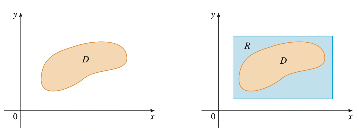
Double Integrals over General Regions

We want to extend the previous idea from region of rectangle (\(R = [a, b] \times [c, d]\)) to a bounded region \(D\) (\(D\) can be enclosed in a rectangular region \(R\)) of more general shape. Then we define a new function \(F\) with domain \(R\) by:

\[ F(x, y)= \begin{cases} f(x, y), & (x, y) \in D\\ 0, \quad & (x, y) \notin D \; \text{ but } \in R \end{cases} \]

If \(F\) is integrable over \(R\), then we define the double integral of $f$ over $D$ by:

\[\underset{D}{\int\int} f(x, y) dA = \underset{R}{\int\int} F(x, y) dA\]

This makes sense because:

1. The rectangle version has been previously defined.
2. \(F(x, y) = 0\) when \((x, y) \notin D\), so it contributes nothing to the integral.

Notice here that \(D\) might have discontinuities at the boundary points. However, if the boundary curve of \(D\) is well-behaved ("Any function for which the mathematical theorem I am about to quote is true, only I don't remember exactly which functions these are"), it can be shown that \(\underset{R}{\int\int} F(x, y) dA\) exists and \(\underset{D}{\int\int} f(x, y) dA\) exists.

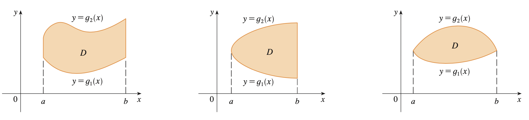
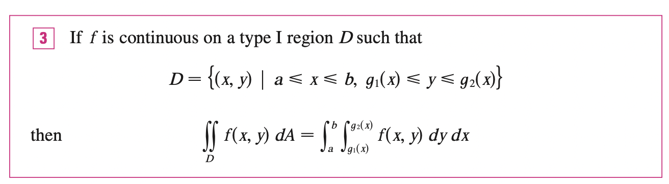
A plane region \(D\) is said to be of type I if it lies between the graphs of two continuous function of \(x\):

\[D = \{(x, y) | a \leq x \leq b, g_1(x) \leq y \leq g_2(x)\}\]

Where \(g_1\), \(g_2\) are continuous on \([a, b]\).

Then:

A plane region \(D\) is said to be of type II if it is defined as:

\[D = \{(x, y) | c \leq y \leq d, h_1(y) \leq x \leq h_2(y)\}\]

Where \(h_1, h_2\) are continuous.

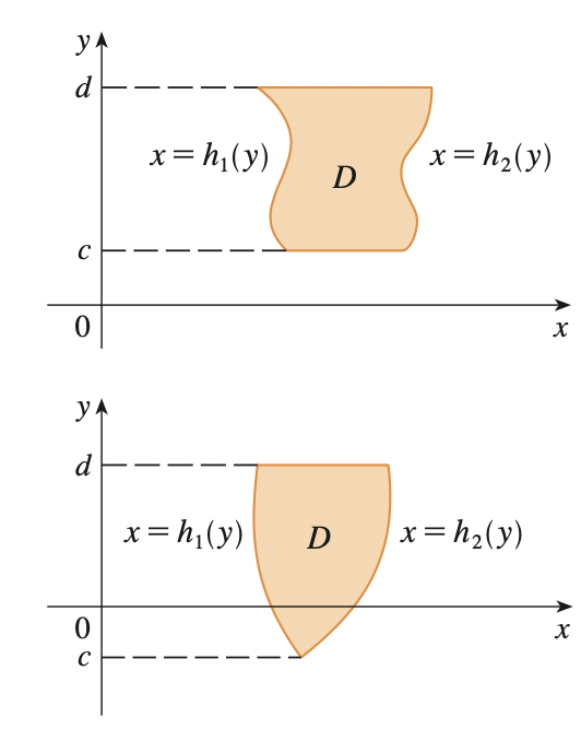
Then:

Properties of Double Expectation

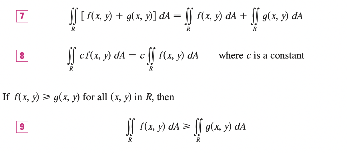
If \(D = D_1 \cup D_2\) where \(D_1\) and \(D_2\) don't overlap except perhaps on their boundaries, then:

\[\underset{D}{\int\int} f(x, y) dA = \underset{D_1}{\int\int} f(x, y) dA + \underset{D_2}{\int\int} f(x, y) dA\]

This property can be used to evaluate double integrals over regions \(D\) that are neither type I nor type II by converting it to regions of type I or type II.

If we integrate the constant function \(f(x, y) = 1\) over a region \(D\), we end up with the area of \(D\):

\[A(D) = \underset{D}{\int\int} 1 dA\]

Surface Area

Triple Integral

Change of Variable

Vector and Matrix Differentiation

Numerator Layout

Let:

\[\mathbf{y} = \psi(\mathbf{x})\]

Where, \(\mathbf{x}, \mathbf{y}\) are column vectors with size \(n, m\) respectively. Then the partial derivative of \(\mathbf{y}\) w.r.t \(\mathbf{x}\) is a \(m \times n\) matrix:

\[ \frac{\partial \mathbf{y}}{\partial \mathbf{x}} = \begin{bmatrix} \frac{\partial y_1}{\partial x_1} & \frac{\partial y_1}{\partial x_2} & .... & \frac{\partial y_1}{\partial x_n}\\ .\\ .\\ .\\ \frac{\partial y_m}{\partial x_1} & \frac{\partial y_m}{\partial x_2} & .... & \frac{\partial y_m}{\partial x_n} \end{bmatrix}_{m \times n} \]

This matrix is called the Jacobian Matrix. Notice that, each row of this matrix is a gradient vector \(\frac{\partial y_1}{\partial \mathbf{x}}\), thus, we can rewrite Jacobian Matrix as:

\[ \frac{\partial \mathbf{y}}{\partial \mathbf{x}} = \begin{bmatrix} \nabla_{\mathbf{x}} y_1\\ .\\ .\\ .\\ \nabla_{\mathbf{x}} y_m \end{bmatrix}_{m \times n} \]

Notice that, single gradient vector \(\nabla_{\mathbf{x}} y_i\) is a row vector, we can represent it as a column vector by

\[\nabla^T_{\mathbf{x}} y_i = \frac{\partial y_i}{\partial \mathbf{x}^T} = (\frac{\partial y_i}{\partial \mathbf{x}})^T\]

At the same time:

\[ \frac{\partial \mathbf{y}}{\partial \mathbf{x}} = \begin{bmatrix} \frac{\partial \mathbf{y}}{\partial x_1} & ..... & \frac{\partial \mathbf{y}}{\partial x_n}\\ \end{bmatrix} \]

Where:

\[ \frac{\partial \mathbf{y}}{\partial x_i} = \begin{bmatrix} \frac{\partial y_1}{\partial x_i}\\ .\\ .\\ .\\ \frac{\partial y_m}{\partial x_i} \end{bmatrix} \]

Denominator Layout

\[\mathbf{y} = \psi(\mathbf{x})\]

Where, \(\mathbf{x}, \mathbf{y}\) are row vectors with size \(n, m\) respectively. Then the partial derivative of \(\mathbf{y}\) w.r.t \(\mathbf{x}\) is a \(n \times m\) matrix:

\[ \frac{\partial \mathbf{y}}{\partial \mathbf{x}} = \begin{bmatrix} \frac{\partial y_1}{\partial x_1} & \frac{\partial y_2}{\partial x_1} & .... & \frac{\partial y_m}{\partial x_1}\\ .\\ .\\ .\\ \frac{\partial y_1}{\partial x_n} & \frac{\partial y_2}{\partial x_n} & .... & \frac{\partial y_m}{\partial x_n} \end{bmatrix}_{n \times m} \]

In terms of gradient vectors (to be consistent with the layout, they are column vectors now. It is possible to represent gradient vectors as row vectors while using denominator layout just by adding transpose to the formula below ):

\[ \frac{\partial \mathbf{y}}{\partial \mathbf{x}} = \begin{bmatrix} \nabla_{\mathbf{x}} y_1 & .... & \nabla_{\mathbf{x}} y_m\\ \end{bmatrix}_{n \times m} \]

At the same time:

\[ \frac{\partial \mathbf{y}}{\partial \mathbf{x}} = \begin{bmatrix} \frac{\partial \mathbf{y}}{\partial x_1} \\ .\\ .\\ .\\ \frac{\partial \mathbf{y}}{\partial x_n}\\ \end{bmatrix} \]

Where \(\frac{\partial \mathbf{y}}{\partial x_i}\) is now a row vector:

\[ \frac{\partial \mathbf{y}}{\partial x_i} = \begin{bmatrix} \frac{\partial y_1}{\partial x_i} & .... & \frac{\partial y_m}{\partial x_i}\\ \end{bmatrix}_{n \times m} \]

Derivative of Function of the Form: \(\; \mathbf{y} = A\mathbf{x}\)

Proof:

Since \(y_i = \sum^{n}_{k=1} a_{ik} x_k \implies \frac{\partial y_i}{\partial x_j} = a_{ij}\)

Thus, the Jacobian Matrix is:

\[ \frac{\partial \mathbf{y}}{\partial \mathbf{x}} = \begin{bmatrix} \nabla_{\mathbf{x}} y_1\\ .\\ .\\ .\\ \nabla_{\mathbf{x}} y_m \end{bmatrix}_{m \times n} = A \]

Now, let \(\mathbf{x} = f(\mathbf{\alpha})\), where \(\mathbf{\alpha}\) is a \(r\) dimensional vector, then the above results can be extended using chain rule:

\[\frac{\partial \mathbf{y}}{\partial \mathbf{r}} = \frac{\partial \mathbf{y}}{\partial \mathbf{x}}\frac{\partial \mathbf{x}}{\partial \mathbf{\alpha}} = [A \frac{\partial \mathbf{x}}{\partial \mathbf{\alpha}}]_{m \times r}\]

Proof:

Since \(y_i = \sum^{n}_{k=1} a_{ik} x_k(\alpha_1, ...., \alpha_r) \implies \frac{\partial y_i}{\partial r_j} = \sum^{n}_{k=1} a_{ik} \frac{\partial y_i}{\partial x_k}\frac{\partial x_k}{\partial \alpha_j} = \sum^{n}_{k=1} a_{ik} \frac{\partial x_k}{\partial \alpha_j}\)

Thus, the Jacobian Matrix is:

\[ \frac{\partial \mathbf{y}}{\partial \mathbf{\alpha}} = \begin{bmatrix} \sum^{n}_{k=1} a_{1k} \frac{\partial x_k}{\partial \alpha_1} & ... & \sum^{n}_{k=1} a_{1k} \frac{\partial x_k}{\partial \alpha_r}\\ .\\ .\\ .\\ \sum^{n}_{k=1} a_{mk} \frac{\partial x_k}{\partial \alpha_1} & ... & \sum^{n}_{k=1} a_{mk} \frac{\partial x_k}{\partial \alpha_r} \end{bmatrix}_{m \times n} = [A \frac{\partial \mathbf{x}}{\partial \mathbf{\alpha}}]_{m \times r} \]

Ref