Value Function Approximation (2)

Value Function Approximation (Algorithms)

Approximate Value Iteration

Population Version

Recall that the procedure for VI is:

$$V_{k+1}\leftarrow T^{\pi }{V}_k$$ $$V_{k+1}\leftarrow T^{\ast }{V}_k$$

One way to develop its approximation version is to perform each step only approximately (i.e find $V_{k+1}\in \mathbf{F}$) such that:

$$V_{k+1}\approx T{V}_k$$

Where $T$ can be $T^{\ast }$ or $T^{\pi }$.

We start from a $V_0\in \mathbf{F}$, and then at each iteration $k$ of AVI, we solve (i.e $p$ is often 2):

$$V_{k+1}\leftarrow \underset{V\in \mathbf{F}}{\arg min}\Vert V-T{V}_k{\Vert }_{p,\mu }^p$$

At each iteration, $T{V}_k$ (our target) may not be within $\mathbf{F}$ anymore even though $V_k\in \mathbf{F}$, we may have some approximation error at each iteration of AVI. The amount of error depends on how expressive $\mathbf{F}$ is and how much $T$ can push a function within $\mathbf{F}$ outside that space.

Batch Version

The objective of AVI cannot be computed because:

• $\mu$ is unknown
• Environment $R,P$ is often not available, thus $T{Q}_k$ cannot be computed.

If we have samples in the form of $(X,A,R,X^{\prime })$, we can compute the unbiased sample of $T{Q}_k$:

$${\hat{T}}^{\pi }{Q}_k=R+\gamma Q(X^{\prime },A^{\prime })$$ $${\hat{T}}^{\ast }{Q}_k=R+\gamma \underset{a^{\prime }\in A}{max}Q(X^{\prime },a^{\prime })$$

Where $A^{\prime }\sim \pi (\cdot |X^{\prime })$

The question is: can we replace $T{Q}_k$ with $\hat{T}{Q}_k$?

Given any $Z=(X,A)$ $$\begin{array}{rl}{E}_{\hat{T}{Q}_k}[|Q(Z)-\hat{T}{Q}_k(Z){|}^2|Z]& =E_{\hat{T}{Q}_k}[|Q(Z)-T{Q}_k(Z)+T{Q}_k(Z)-\hat{T}{Q}_k(Z){|}^2|Z]\\ & =E_{\hat{T}{Q}_k}[|Q(Z)-T{Q}_k(Z){|}^2|Z]+E_{\hat{T}{Q}_k}[|T{Q}_k(Z)-\hat{T}{Q}_k(Z){|}^2|Z]+2E_{\hat{T}{Q}_k}[(Q(Z)-T{Q}_k(Z))(T{Q}_k(Z)-\hat{T}{Q}_k(Z))|Z]\\ & =E_{\hat{T}{Q}_k}[|Q(Z)-T{Q}_k(Z){|}^2|Z]+E_{\hat{T}{Q}_k}[|T{Q}_k(Z)-\hat{T}{Q}_k(Z){|}^2|Z]\end{array}$$

Since $Z\sim \mu$:

$$\begin{array}{rl}{E}_{\mu }[E_{\hat{T}{Q}_k}[|Q(Z)-T{Q}_k(Z){|}^2|Z]+E_{\hat{T}{Q}_k}[|T{Q}_k(Z)-\hat{T}{Q}_k(Z){|}^2|Z]]& =E_{\mu ,\hat{T}{Q}_k}[|Q(Z)-T{Q}_k(Z){|}^2]+E_{\mu ,\hat{T}{Q}_k}[|T{Q}_k(Z)-\hat{T}{Q}_k(Z){|}^2]\\ & =\Vert Q(Z)-T{Q}_k(Z){\Vert }_{2,\mu }^2+E_{\mu }[Var[\hat{T}{Q}_k(Z)|Z]]\end{array}$$

Since the expectation of variance term does not depend on $Q$, the solution to the surrogate objective is the same as the original objective:

$$\underset{Q\in \mathbf{F}}{\arg min}{E}_{\mu ,\hat{T}{Q}_k}[|Q(Z)-\hat{T}{Q}_k(Z){|}^2]=\underset{Q\in \mathbf{F}}{\arg min}\Vert Q(Z)-T{Q}_k(Z){\Vert }_{2,\mu }^2$$

Similar to ERM, we do not know the environment dynamics $R,P$ and distribution $\mu$. We can use samples and estimate the expectation:

$$\frac{1}{N}\sum _{i=1}^N|Q(X_i,A_i)-\hat{T}{Q}_k(X_i,A_i){|}^2=\Vert Q-\hat{T}{Q}_k{\Vert }_{2,D_n}^2$$

This is the basis of DQN.

Bellman Residual Minimization

Population Version

Recall that:

$$V=T^{\pi }V⟹V=V^{\pi }$$

Under FA, we may not achieve this exact equality, instead:

$$V\approx V^{\pi }$$

Thus, we can formulate our objective:

$$V=\underset{V\in \mathbf{F}}{\arg min}\Vert V-T^{\pi }V{\Vert }_{p,\mu }^p=\Vert BR(V){\Vert }_{p,\mu }^p$$

By minimizing this objective ($p$ is usually 2), we have Bellman Residual Minimization.

This procedure is different from AVI in that we do not mimic the iterative process of VI (which is convergent in the exact case without any FA), but instead directly go for the solution of fixed-point equation ($V-T^{\pi }V$ instead of $V-T^{\pi }{V}_k$).

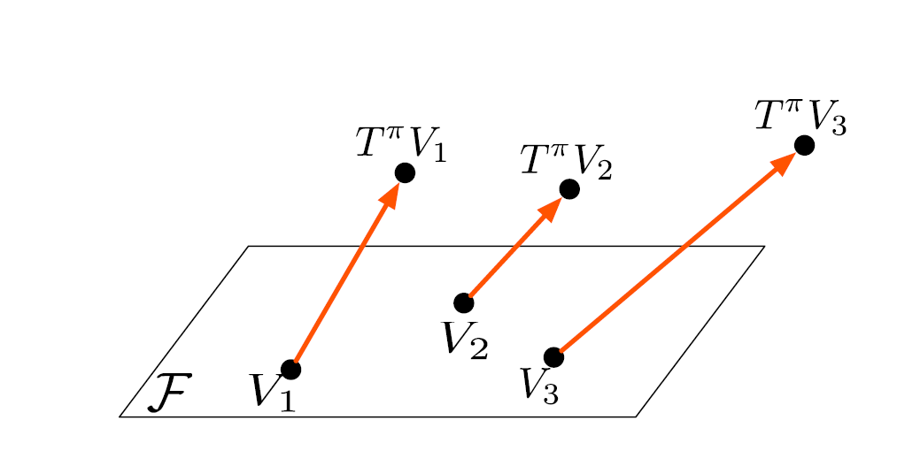
If there exists a $V\in \mathbf{F}$ that makes $\Vert V-T^{\pi }V{\Vert }_{2,\mu }^2=0$ and if we assume $\mu (x)>0,\mathrm{\forall }x\in \chi$, we can conclude that $V(x)=V^{\pi }(x),\mathrm{\forall }x\in \chi$ so $V=V^{\pi }$.

Batch Version

Similar to AVI, we may want to replace $TV$ or $TQ$ by $\hat{T}Q$. Thus, our empirical objective is:

$$Q=\underset{Q\in \mathbf{F}}{\arg min}\frac{1}{N}\sum _{i=1}^N|Q(X_i,A_i)-{\hat{T}}^{\pi }Q(X_i,A_i){|}^2=\Vert Q-{\hat{T}}^{\pi }Q{\Vert }_{2,D_n}^2$$

Using $D_n=\{(X_i,A_i,R_i,X_i^{\prime }){\}}_{i=1}^N$

We can see that $Q$ appears in both ${\hat{T}}^{\pi }Q$ and $Q$, which is different from AVI and ERM. This causes an issue: the minimizer of $\Vert Q-T^{\pi }Q{\Vert }_{2,\mu }^2$ and $\Vert Q-{\hat{T}}^{\pi }Q{\Vert }_{2,\mu }^2$ are not necessarily the same for stochastic dynamics.

To see this, for any $Q$ and $Z=(X,A)$ we compute:

$$E_{{\hat{T}}^{\pi }Q}[|Q(Z)-\hat{T}Q(Z){|}^2|Z]$$

Then:

$$\begin{array}{rl}{E}_{{\hat{T}}^{\pi }Q}[|Q(Z)-{\hat{T}}^{\pi }Q(Z){|}^2|Z]& =E_{{\hat{T}}^{\pi }Q}[|Q(Z)-T^{\pi }Q(Z)+T^{\pi }Q(Z)-{\hat{T}}^{\pi }Q(Z){|}^2|Z]\\ & =E_{{\hat{T}}^{\pi }Q}[|Q(Z)-T^{\pi }Q(Z){|}^2|Z]+E_{{\hat{T}}^{\pi }Q}[|T^{\pi }Q(Z)-{\hat{T}}^{\pi }Q(Z){|}^2|Z]+2E_{{\hat{T}}^{\pi }Q}[(Q(Z)-T^{\pi }Q(Z))(T^{\pi }Q(Z)-{\hat{T}}^{\pi }Q(Z))|Z]\\ & =E_{{\hat{T}}^{\pi }Q}[|Q(Z)-T^{\pi }Q(Z){|}^2|Z]+E_{{\hat{T}}^{\pi }Q}[|T^{\pi }Q(Z)-{\hat{T}}^{\pi }Q(Z){|}^2|Z]\end{array}$$

Since $Z\sim \mu$, the first term is:

$$E_{{\hat{T}}^{\pi }Q,\mu }[|Q(Z)-T^{\pi }Q(Z){|}^2]=\Vert Q-T^{\pi }Q{\Vert }_{2,\mu }^2$$

The second term is:

$$E_{\mu }[E_{{\hat{T}}^{\pi }Q}[|T^{\pi }Q(Z)-{\hat{T}}^{\pi }Q(Z){|}^2|Z]]=E_{\mu }[Var[{\hat{T}}^{\pi }Q(Z)|Z]]$$

We can see that the variance term $Var[{\hat{T}}^{\pi }Q(Z)$ depends on $Q$, as we minimize the objective w.r.t $Q$ in stochastic dynamical systems (for deterministic ones, it is zero), we have $E_{}[Var{[}^{}Q(Z)|Z]]$, so the minimizer of the batch version objective is not the same as population version for BRM in stochastic dynamics.

Projected Bellman Error

From BRM, we know that even though $V\in \mathbf{F}$, $T^{\pi }V$ may not be in $\mathbf{F}$. Thus, a good approximator $V\in \mathbf{F}$ should have distance to $T^{\pi }V$ small. Thus, we want to find $V\in \mathbf{F}$ such that $V$ is the projection of $T^{\pi }V$ onto the space $\mathbf{F}$.

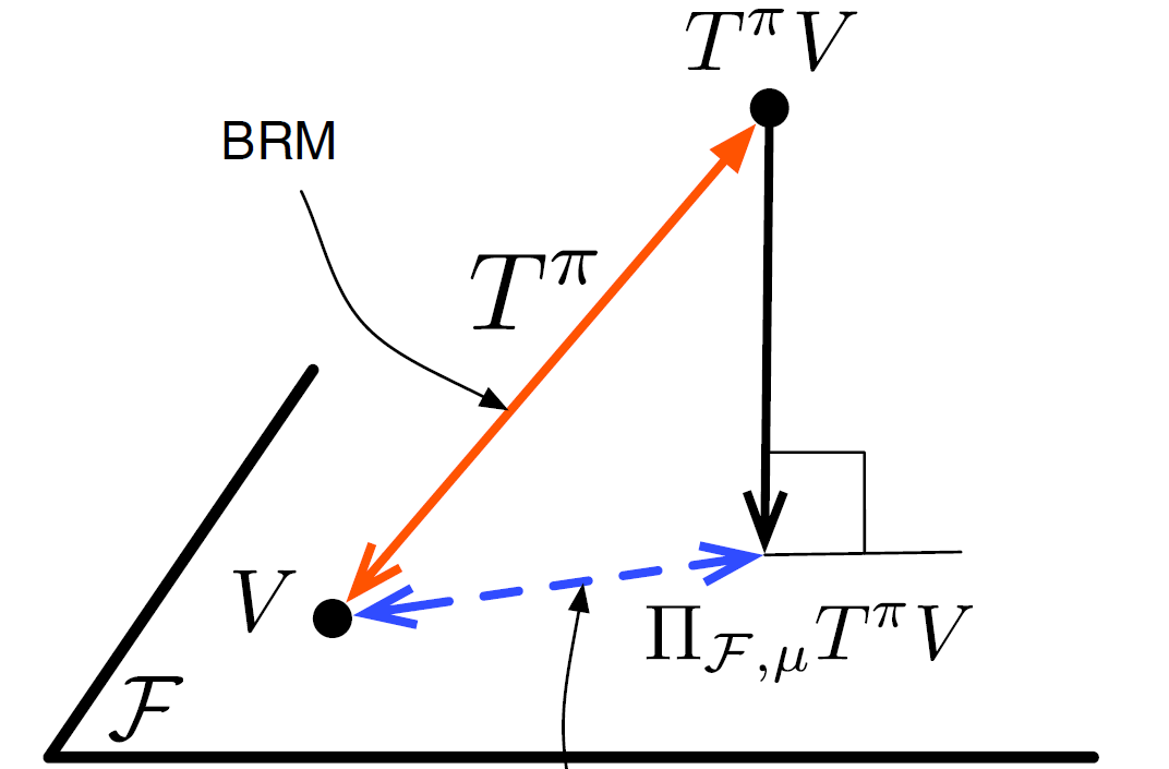
We want to find a $V\in \mathbf{F}$ such that:

$$V=\prod _{\mathbf{F},\mu }{T}^{\pi }V$$

Where $\prod _{\mathbf{F},\mu }$ is the projection operator.

TRhe projectio operator $\prod _{\mathbf{F},\mu }$ is a linear operator that takes $V\in B(\chi )$ and maps it to closest point on $F$ measured according to its $L_2(\mu )$ norm:

$$\prod _{\mathbf{F},\mu }V\triangleq \underset{V^{\prime }\in \mathbf{F}}{\arg min}\Vert V^{\prime }-V{\Vert }_{2,\mu }^2$$

It has some properties:

1. The projection belongs to function space $\mathbf{F}$: $$\prod _{\mathbf{F},\mu }V\in \mathbf{F}$$
2. If $V\in \mathbf{F}$, the projection is itself: $$V\in \mathbf{F}⟹\prod _{\mathbf{F},\mu }V=V$$
3. The projection operator onto a subspace is a non-expansion: $$\Vert \prod _{\mathbf{F},\mu }{V}_1-\prod _{\mathbf{F},\mu }{V}_2{\Vert }_{2,\mu }^2\le \Vert V_1-V_2{\Vert }_{2,\mu }^2$$

Population Version

We can define a loss function based on $V=\prod _{\mathbf{F},\mu }{T}^{\pi }V$:

$$\Vert V-\prod _{\mathbf{F},\mu }{T}^{\pi }V{\Vert }_{2,\mu }^2$$

This is called Projected Bellman Error or Mean Square Projected Bellman Error.

We find the value function by solving the following optimization problem:

$$V=\underset{V\in \mathbf{F}}{\arg min}\Vert V-\prod _{\mathbf{F},\mu }{T}^{\pi }V{\Vert }_{2,\mu }^2$$

Since $V\in \mathbf{F}$, the projection operator is linear:

$$\begin{array}{rl}V-\prod _{\mathbf{F},\mu }{T}^{\pi }V& =\prod _{\mathbf{F},\mu }V-\prod _{\mathbf{F},\mu }{T}^{\pi }V\\ & =\prod _{\mathbf{F},\mu }(V-T^{\pi }V)\\ & =-\prod _{\mathbf{F},\mu }(T^{\pi }V-V)\\ & =-\prod _{\mathbf{F},\mu }(BR(V))\end{array}$$

So the objective can be rewritten as:

$$V=\underset{V\in \mathbf{F}}{\arg min}\Vert \prod _{\mathbf{F},\mu }BR(V){\Vert }_{2,\mu }^2$$

Which is the norm of the projection of the Bellman Residual onto $\mathbf{F}$.

We can think of solving the projected bellman error objective as solving the two coupled optimization problems:

1. Find the projection point given value function $V^{\prime }$: $$V^{\prime \prime }=\underset{V^{\prime \prime }\in \mathbf{F}}{\arg min}\Vert V^{\prime \prime }-T^{\pi }{V}^{\prime }{\Vert }_{2,\mu }^2$$
2. Find the value function $V^{\prime }$ on $\mathbf{F}$ that is closest to the projection point $V^{\prime \prime }$: $$V^{\prime }=\underset{V^{\prime }\in \mathbf{F}}{\arg min}\Vert V^{\prime }-V^{\prime \prime }{\Vert }_{2,\mu }^2$$

Least Square Temporal Difference Learning (Population Version)

If $\mathbf{F}$ is a linear FA with basis functions ${\varphi }_1,....,{\varphi }_p$:

$$\mathbf{F}:\{x\to \mathit{\varphi }(x{)}^T\mathbf{w};\mathbf{w}\in {\mathbb{R}}^p\}$$

We can find a direct solution to the PBE objective, that is we want to find $V\in \mathbf{F}$ s.t:

$$V=\prod _{\mathbf{F},\mu }{T}^{\pi }V$$

We assume that:

• $\chi$ is finite and $|\chi |=N$, $N\gg p$, each ${\mathit{\varphi }}_i=[{\varphi }_i(x_1)....{\varphi }_i(x_N){]}^T$ is a $N$-dimentional vector.

Then, we define ${\mathrm{\Phi }}_{N\times p}$ as the matrix of concatenating all features:

$$\mathrm{\Phi }=[{\mathit{\varphi }}_1....{\mathit{\varphi }}_p{]}_{N\times p}$$

The value function $V\in \mathbf{F}$ is then:

$$V_{N\times 1}={\mathrm{\Phi }}_{N\times p}{\mathbf{w}}_{p\times 1}$$

Our goal is to find a weight vector $\mathbf{w}\in {\mathbb{R}}^p$ such that:

$$V=\prod _{\mathbf{F},\mu }{T}^{\pi }V⟹\mathrm{\Phi }\mathbf{w}=\prod _{\mathbf{F},\mu }{T}^{\pi }(\mathrm{\Phi }\mathbf{w})$$

Let $M=\text{diag}(\mu )$, since:

$$\Vert V{\Vert }_{2,\mu }^2=<V,V{>}_{\mu }=\sum _{x\in \chi }|V(x){|}^2\mu (x)=V^{T}MV$$

$$<V_1,V_2{>}_{\mu }=\sum _{x\in \chi }{V}_1(x)V_2(x)=V_1^{T}M{V}_2$$

Then, the projection operator onto the linear $\mathbf{F}$ would be:

$$\begin{array}{rl}\prod _{\mathbf{F},\mu }V& =\underset{V^{\prime }\in \mathbf{F}}{\arg min}\Vert V^{\prime }-V{\Vert }_{2,\mu }^2\\ & =\underset{\mathbf{w}\in {\mathbb{R}}^p}{\arg min}\Vert \mathrm{\Phi }\mathbf{w}-V{\Vert }_{2,\mu }^2\\ & =\underset{\mathbf{w}\in {\mathbb{R}}^p}{\arg min}(\mathrm{\Phi }\mathbf{w}-V{)}^{T}M(\mathrm{\Phi }\mathbf{w}-V)\end{array}$$

By taking the derivative and setting it to zero (assuming that ${\mathrm{\Phi }}^{T}M\mathrm{\Phi }$ is invertible):

$$\frac{\partial \prod _{\mathbf{F},\mu }V}{\partial \mathbf{w}}={\mathrm{\Phi }}^{T}M(\mathrm{\Phi }\mathbf{w}-V)=0$$ $$⟹{\mathbf{w}}^{\mathbf{\ast }}=({\mathrm{\Phi }}^{T}M\mathrm{\Phi }{)}^{-1}{\mathrm{\Phi }}^{T}MV$$

Then the projection is:

$$\prod _{\mathbf{F},\mu }V=\mathrm{\Phi }\mathbf{w}=\mathrm{\Phi }({\mathrm{\Phi }}^{T}M\mathrm{\Phi }{)}^{-1}{\mathrm{\Phi }}^{T}MV$$

Since $T^{\pi }V=r^{\pi }(x)+\gamma \sum _{x\in \chi ,a\in \mathbf{A}}{P}^{\pi }(x^{\prime }|x,a)\pi (a|s)V(x^{\prime })$, we can write it in vector form for all states:

$$(T^{\pi }V{)}_{N\times 1}={\mathbf{r}}_{N\times 1}^{\pi }+\gamma P_{N\times N}^{\pi }{V}_{N\times 1}$$ $$⟹(T^{\pi }\mathrm{\Phi }\mathbf{w}{)}_{N\times 1}={\mathbf{r}}_{N\times 1}^{\pi }+\gamma P_{N\times N}^{\pi }{\mathrm{\Phi }}_{N\times p}{\mathbf{w}}_{p\times 1}$$

Substitute the equation of $T^{\pi }\mathrm{\Phi }\mathbf{w}$ into $V$ in the projection equation:

$$\prod _{\mathbf{F},\mu }{T}^{\pi }\mathrm{\Phi }\mathbf{w}=\mathrm{\Phi }\mathbf{w}=\mathrm{\Phi }({\mathrm{\Phi }}^{T}M\mathrm{\Phi }{)}^{-1}{\mathrm{\Phi }}^{T}M(T^{\pi }\mathrm{\Phi }\mathbf{w})$$ $$⟹\mathrm{\Phi }\mathbf{w}=[\mathrm{\Phi }({\mathrm{\Phi }}^{T}M\mathrm{\Phi }{)}^{-1}{\mathrm{\Phi }}^{T}M][{\mathbf{r}}^{\pi }+\gamma P^{\pi }\mathrm{\Phi }\mathbf{w}]$$

Multiply both sides by ${\mathrm{\Phi }}^{T}M$ and simply:

$${\mathrm{\Phi }}^{T}M\mathrm{\Phi }\mathbf{w}=[{\mathrm{\Phi }}^{T}M\mathrm{\Phi }({\mathrm{\Phi }}^{T}M\mathrm{\Phi }{)}^{-1}{\mathrm{\Phi }}^{T}M][{\mathbf{r}}^{\pi }+\gamma P^{\pi }\mathrm{\Phi }\mathbf{w}]$$ $$⟹{\mathrm{\Phi }}^{T}M\mathrm{\Phi }\mathbf{w}={\mathrm{\Phi }}^{T}M[{\mathbf{r}}^{\pi }+\gamma P^{\pi }\mathrm{\Phi }\mathbf{w}]$$ $$⟹{\mathrm{\Phi }}^{T}M\mathrm{\Phi }\mathbf{w}-{\mathrm{\Phi }}^{T}M[{\mathbf{r}}^{\pi }+\gamma P^{\pi }\mathrm{\Phi }\mathbf{w}]=0$$ $$⟹{\mathrm{\Phi }}^{T}M[{\mathbf{r}}^{\pi }+\gamma P^{\pi }\mathrm{\Phi }\mathbf{w}-\mathrm{\Phi }\mathbf{w}]=0$$ $$⟹{\mathbf{w}}_{TD}=[{\mathrm{\Phi }}^{T}M(\mathrm{\Phi }-\gamma P^{\pi }\mathrm{\Phi }){]}^{-1}{\mathrm{\Phi }}^{T}M{\mathbf{r}}^{\pi }$$

The solution ${\mathbf{w}}_{TD}$ is called Least Square Temporal Difference Method (LSTD).

Notice that the term ${\mathbf{r}}^{\pi }+\gamma P^{\pi }\mathrm{\Phi }\mathbf{w}-\mathrm{\Phi }\mathbf{w}=T^{\pi }V-V=BR(V)$. Hence:

$${\mathrm{\Phi }}^{T}M(BR(V))=0$$ $$⟹<{\varphi }_i,BR(V)>=0$$

Thus, LSTD finds a $\mathbf{w}$ s.t the Bellman Residual is orthogonal to the basis of $\mathbf{F}$ which is exactly what we want.

Batch Version

We have showed that the solution to $V=\prod _{\mathbf{F},\mu }{T}^{\pi }V$ with linear FA $V=\mathrm{\Phi }\mathbf{w}$ is:

$${\mathbf{w}}_{TD}=A_{p\times p}^{-1}{\mathbf{b}}_{p\times 1}$$

Where:

• $A^{-1}={\mathrm{\Phi }}^{T}M(\mathrm{\Phi }-\gamma P^{\pi }\mathrm{\Phi }){]}^{-1}$
• $\mathbf{b}={\mathrm{\Phi }}^{T}M{\mathbf{r}}^{\pi }$

Expand $A$ and $\mathbf{b}$ in terms of summations, we have:

$$A_{ij}=\sum _{n=1}^N{\mathrm{\Phi }}_{in}^T\mu (n)(\mathrm{\Phi }-\gamma P^{\pi }\mathrm{\Phi }{)}_{ij}$$ $$b_i=\sum _{n=1}^N{\mathrm{\Phi }}_{in}^T\mu (n)r_n^{\pi }$$

Thus, in terms of current state $x$ and next state $x^{\prime }$:

$$A=\sum _{x\in \chi }\mu (x)\mathit{\varphi }(x)[\mathit{\varphi }(x)-\gamma \sum _{x^{\prime }\in \chi }{P}^{\pi }(x^{\prime }|x)\mathit{\varphi }(x^{\prime }){]}^T=E_{\mu }[\mathit{\varphi }(X)[\mathit{\varphi }(X)-\gamma E_{P^{\pi }}[\mathit{\varphi }(X^{\prime })]{]}^T]$$

$$\mathbf{b}=\sum _{x\in \chi }\mu (x)\mathit{\varphi }(x)r^{\pi }(x)=E_{\mu }[\mathit{\varphi }(X)r^{\pi }(X)]$$

Given data set $D_n=\{X_i,R_i,X_i^{\prime }{\}}_{i=1}^M$ with $X_i\sim \mu$, $X^{\prime }\sim P^{\pi }(\cdot |X_i)$ and $R_i\sim R^{\pi }(\cdot |X_i)$, we define the empirical estimator ${\hat{A}}_n,{\hat{\mathbf{b}}}_n$ as:

$${\hat{A}}_n=\frac{1}{M}\sum _{i=1}^M\mathit{\varphi }(X_i)[\mathit{\varphi }(X_i)-\gamma \mathit{\varphi }(X_i^{\prime }){]}^T$$ $${\hat{\mathbf{b}}}_n=\frac{1}{M}\sum _{i=1}^M\mathit{\varphi }(X)R_i$$

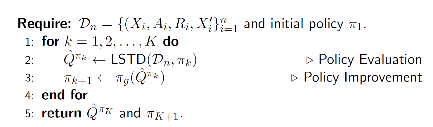
We can use LSTD to define an approximate policy iteration procedure to obtain a close to optimal policy (LSPI):

Semi-Gradient TD

Suppose that we know the true value function $V^{\pi }$ and we want to find an approximation $\hat{V}$, parameterized by $\mathbf{w}$. The population loss:

$$V=\underset{\hat{V}\in \mathbf{F}}{\arg min}\frac{1}{2}\Vert V^{\pi }-\hat{V}{\Vert }_{2,\mu }^2$$

Using samples $X_t\sim \mu$, we can define an SGD procedure that updates ${\mathbf{w}}_t$ as follows:

$$\begin{array}{rl}{\mathbf{w}}_{t+1}& \leftarrow {\mathbf{w}}_t-{\alpha }_t{\mathrm{\nabla }}_{{\mathbf{w}}_t}[\frac{1}{2}|V^{\pi }(X_t)-\hat{V}(X_t;{\mathbf{w}}_t){|}^2]\\ & ={\mathbf{w}}_t+{\alpha }_t(V^{\pi }(X_t)-\hat{V}(X_t;{\mathbf{w}}_t)){\mathrm{\nabla }}_{{\mathbf{w}}_t}\hat{V}(X_t;{\mathbf{w}}_t)\end{array}$$

If we select proper step size ${\alpha }_t$, then the SGD converges to the stationary point.

When we do not know $V^{\pi }$, we can use bootstrapped estimate (TD estimate ${\hat{T}}^{\pi }{V}_t$) instead:

$${\mathbf{w}}_{t+1}\leftarrow {\mathbf{w}}_t+{\alpha }_t({\hat{T}}^{\pi }{V}_t-\hat{V}(X_t;{\mathbf{w}}_t)){\mathrm{\nabla }}_{{\mathbf{w}}_t}\hat{V}(X_t;{\mathbf{w}}_t)$$ $${\mathbf{w}}_{t+1}\leftarrow {\mathbf{w}}_t+{\alpha }_t(R_t+\hat{V}(X_t^{\prime };{\mathbf{w}}_t)-\hat{V}(X_t;{\mathbf{w}}_t)){\mathrm{\nabla }}_{{\mathbf{w}}_t}\hat{V}(X_t;{\mathbf{w}}_t)$$

The substitution of $V^{\pi }(X_t)$ with ${\hat{T}}^{\pi }{V}_t(X_t)$ does not follow from the SGD of any loss function. The TD update is note a true SGD update, that is, we call it a semi-gradient update.