probability-3

Statistics Inference

Sampling and Statistics

In a typical statistical problem, we have \(p_X(x), f_X(x)\) unknown. Our ignorance about the \(p_X(x), f_X(x)\) can roughly be classified in one of two ways:

1. \(f(x)\) or \(p_X(x)\) is completely unknown.
2. The form of \(f_X(x)\) or \(p_X(x)\) is known down to an unknown parameter vector \(\mathbf{\theta}\).

We will focus on the second case. We often denote this problem by saying that the random variable \(X\) has density or mass function of the form \(f_{X}(x; \theta)\) or \(p_X(x;\theta)\), where \(\theta \in \Omega\) for a special parameter space \(\Omega\). Since \(\theta\) is unknown, we want to estimate it.

In the process, our information about case 1 or 2 comes from a sample on \(X\). The sample observations have the same distribution as \(X\), and we denote them as \(X_1, ...., X_n\) where \(n\) is the sample size. When the sample is actually drawn, we use lower case letters to represent the realization \(x_1, ..., x_n\) of random samples.

Once the sample is drawn, then \(t\) is called the realization of \(T\), where \(t = T(x_1, ...., x_n)\).

Point Estimators

Continue from above formulation, the problem of case 2 can be phrased as:

Let \(X_1, ...., X_n\) be a random sample on a random variable \(X\) with a density or mass function of the form \(f_X(x; \theta)\) or \(p_X (x; \theta)\). In this situation, an point estimator of \(\theta\) is a statistic \(T\). While we call \(T\) an estimator of \(\theta\), we call \(t\) an estimate of \(\theta\).

In our problem, the information in the sample and the parameter \(\theta\) are involved in the joint distribution of the random sample (i.e \(\prod^{n}_{i=1} f(x_1 ; \theta)\)). We want to view this as a function of \(\theta\):

\[L(\theta) = L(\theta; x_1, ....., x_n) = \prod^{n}_{i=1} f_X(x_i; \theta)\]

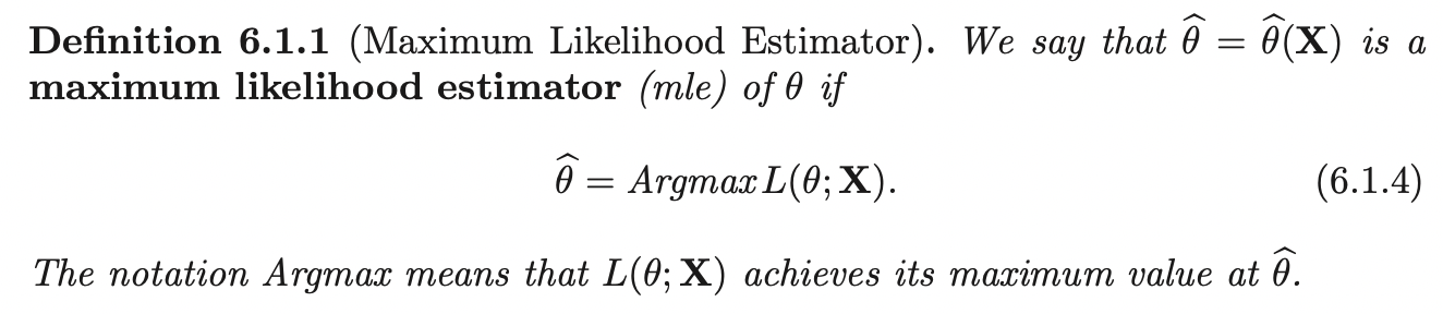
This is called the likelihood function of the random sample. As an estimate of \(\theta\), an often-used estimate is the value of \(\theta\) that provides a maximum of \(L(\theta)\). If it is unique, this is called the Maximum likelihood estimator and we denote it as \(\hat{\theta}\):

\[\hat{\theta} = \arg\max_{\theta} L(\theta; \mathbf{X})\]

If \(\theta\) is a vector of parameters, this results in a system of equations to be solved simultaneously called estimating equations.

The Method of Monte Carlo

Bootstrap Procedures

Consistency and Limiting Distributions

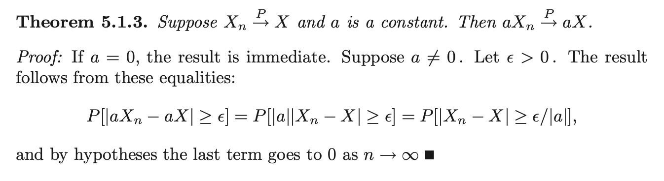
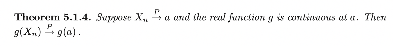
Convergence in Probability

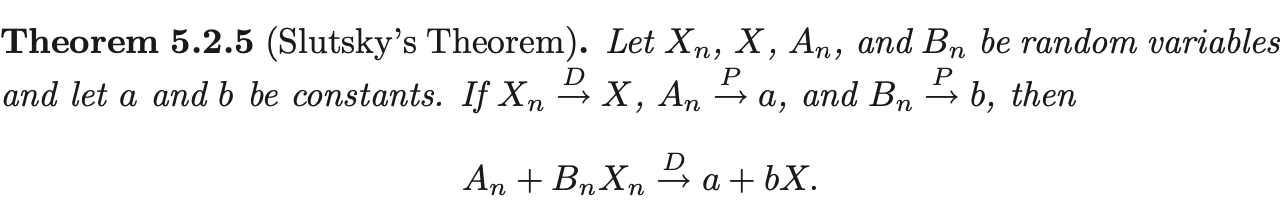
We formalize a way of saying that a sequence of random variables \(\{X_n\}\) is getting "close" to another random variable \(X\) as \(n \rightarrow \infty\) by:

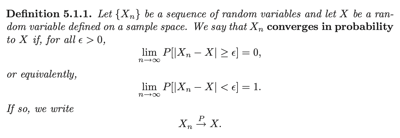
In statistics, \(X\) is often a constant (i.e \(X\) is a degenerate random variable with all its mass at some constant \(a\)). In this case, we write \(X_n \overset{P}{\rightarrow} a\).

Weak Law of Large Numbers

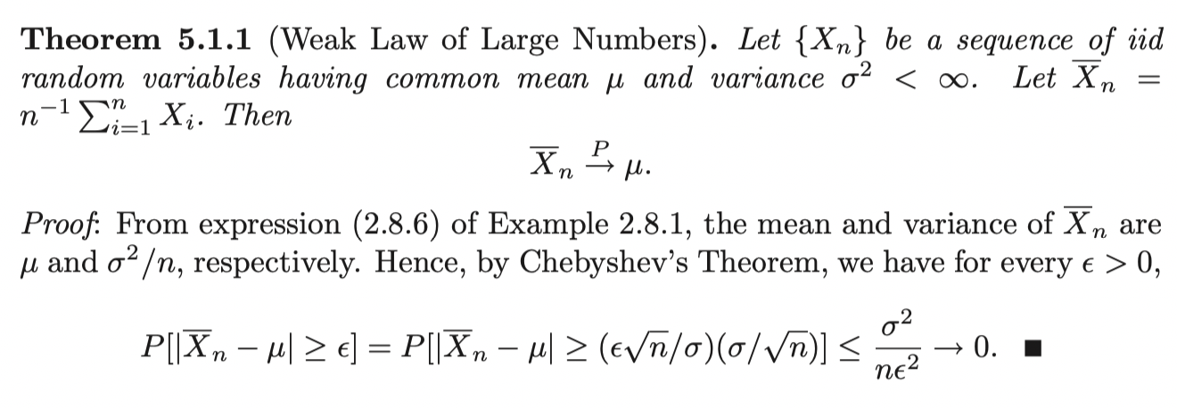
This theorem says that all the mass of the distribution of \(\bar{X}_n\) is converging to a constant \(\mu\), as \(n \rightarrow \infty\).

Consistency

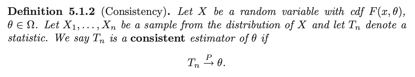
If \(X_1, ..., X_n\) is a random sample from a distribution with finite mean \(\mu\) and variance \(\sigma^2\), then by the weak law of large numbers, the sample mean \(\bar{X}_n\) is a consistent estimator of \(\mu\).

Convergence in Distribution

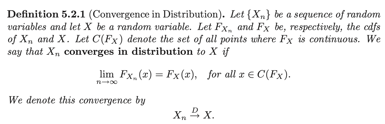
Often, we say that the distribution of \(X\) is the asymptotic distribution or limiting distribution of sequence \(\{X_n\}\). In general, we can represent \(X\) by the distribution it follows, for example:

\[X_n \overset{D}{\rightarrow} N(0, 1)\]

The thing on the right hand side is not a random variable, but a distribution, this is just a convention saying the same thing. In addition, we may say that \(X_n\) has a limiting standard normal distribution to mean the same thing (i.e \(X_n \overset{D}{\rightarrow} N(0, 1)\)).

Convergence in probability is a way of saying that a sequence of random variables \(X_n\) is getting close to another random variable \(X\). On the other hand, convergence in distribution only concerned with the cdfs \(F_{X_n}\) and \(F_X\) (In general, we cannot determine the limiting distribution by considering pmfs or pdfs).

Example:

Let \(X\) be a continuous random variable with a pdf \(f_X (x)\) that is symmetric about 0 (i.e \(f_X(-x) = f_X(x)\)). Then it is easy to show that the density of the random variable \(-X\) and \(X\) have the same distributions (i.e \(F_{-X}(x) = F_X(x)\)). Define the sequence of random variables \(X_n\) as: \[ X_n = \begin{cases} X, \quad & \text{if $n$ is odd}\\ -X, \quad & \text{if $n$ is even}\\ \end{cases} \] Clearly, \(F_{X_n} (x) = F_{X} (x)\) so \(X_n \overset{D}{\rightarrow} X\), but \(X_n\) does not converge in probability to \(X\).

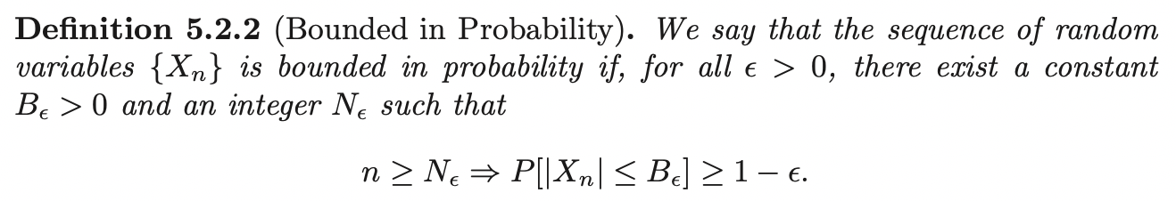
Bounded in Probability

Central Limit Theorem

Maximum Likelihood Methods

Maximum Likelihood Estimation (Single Parameter)

Suppose we have a random sample \(X_1, ...., X_n\) on \(X\) with common pdf \(f(x;\theta)\). Assume that \(\theta\) is a scalar and unknown. The likelihood function is given by:

\[L(\theta; \mathbf{x}) = \prod^{n}_{i=1} f(x_i;\theta)\]

The log likelihood function:

\[l(\theta; \mathbf{x}) = \sum^{n}_{i=1} \log f(x_i;\theta)\]

Then the point estimator (before the observation of \(\mathbf{x}\)) of \(\theta\) is \(\hat{\theta} = \arg\max_{\theta} L(\theta; \mathbf{X})\). We call \(\hat{\theta}\) the ML estimator of \(\theta\). If we have the observation \(\mathbf{x}\), we call \(\hat{\theta} (\mathbf{x})\) the ML estimate.

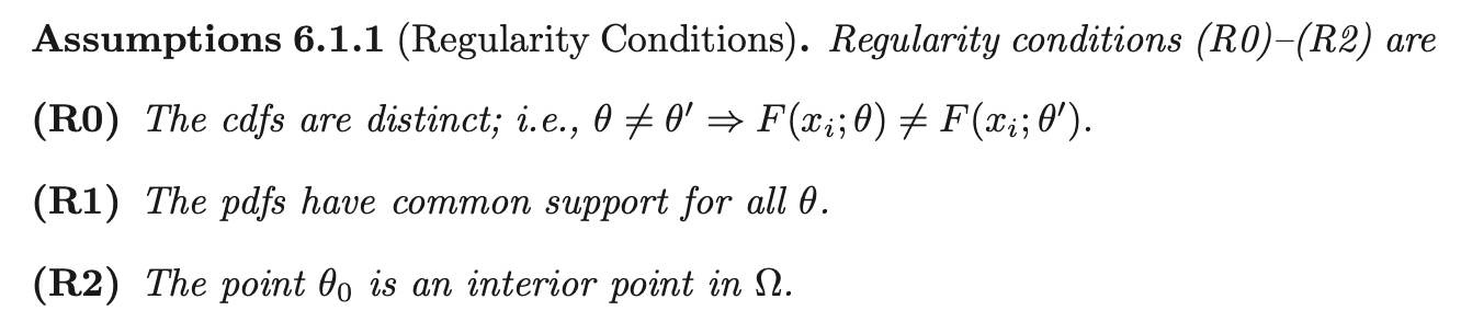
Assumption 1 assumes that the parameter identifies the pdf. The second assumption implies that the support of \(X_i\) does not depend on \(\theta\).

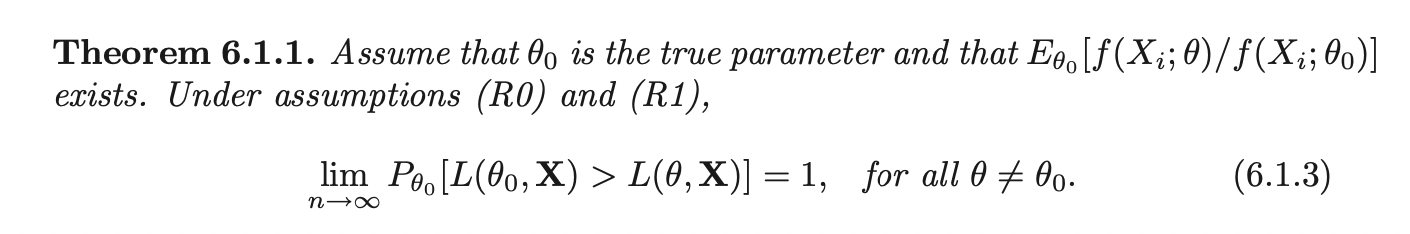
The theorem shows that the maximum of \(L(\theta; \mathbf{X})\) asymptotically separates the true model at \(\theta_0\) from models at \(\theta \neq \theta_0\).

Proof:

Assume \(\theta_0\) is the true parameter value. Then the inequality we want to show \(L(\theta_0; \mathbf{X}) > L(\theta; \mathbf{X})\) can be written as:

\[\frac{1}{n}\sum^{n}_{i=1} \log[f_X(X_i; \theta_0)] > \frac{1}{n}\sum^{n}_{i=1} \log[f_X(X_i; \theta)] \implies \frac{1}{n}\sum^{n}_{i=1} \log[\frac{f_X(X_i; \theta)}{f_X(X_i; \theta_0)}] > 0\]

By the Weak law of large numbers, we have: \[\frac{1}{n}\sum^{n}_{i=1} -\log[\frac{f_X(X_i; \theta)}{f_X(X_i; \theta_0)}] \; \overset{p}{\rightarrow} \; E_{P_X(\cdot | \theta_0)} [ -\log[\frac{f_X(X_i; \theta)}{f_X(X_i; \theta_0)}]]\]

Since the \(-\log\) function is convex, we can apply jensen's inequality \[\frac{1}{n}\sum^{n}_{i=1} -\log[\frac{f_X(X_i; \theta)}{f_X(X_i; \theta_0)}] \; \overset{p}{\rightarrow} \; E_{P_X(\cdot | \theta_0)} [ -\log[\frac{f_X(X_i; \theta)}{f_X(X_i; \theta_0)}]] \geq -\log (E_{P_X(\cdot | \theta_0)} [\frac{f_X(X_i; \theta)}{f_X(X_i; \theta_0)}])\]

But, the expectation is 1:

\[\int_{x} \frac{f_X(x_i; \theta)}{f_X(x_i; \theta_0)} {f_X(x_i; \theta_0)} dx = 1\]

So, we have: \[\frac{1}{n}\sum^{n}_{i=1} -\log[\frac{f_X(X_i; \theta)}{f_X(X_i; \theta_0)}] \geq 0\]

Then: \[\frac{1}{n}\sum^{n}_{i=1} \log[f_X(X_i; \theta_0)] > \frac{1}{n}\sum^{n}_{i=1} \log[f_X(X_i; \theta)] \implies L(\theta_0; \mathbf{X}) > L(\theta; \mathbf{X})\]

As \(n \rightarrow \infty\) the above inequality holds.

That is, asymptotically the likelihood function is maximized at the value \(\theta_0\). So in considering estimates of \(\theta_0\), it is natural to consider the value of \(\theta\) that maximizes the likelihood.

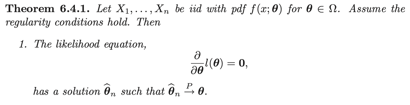
Maximum Likelihood Estimation (Multiple Parameters)

Let \(X_1, ...., X_n\) be i.i.d with common pdf \(f(x; \boldsymbol{\theta})\), where \(\boldsymbol{\theta} \in \Omega \subset \mathbb{R}^p\). The likelihood function is given by:

\[L(\boldsymbol{\theta}; \mathbf{x}) = \prod^{n}_{i=1} f_{X}(x_i; \boldsymbol{\theta})\]

\[l(\boldsymbol{\theta}) = \log L(\boldsymbol{\theta}; \mathbf{x}) = \sum^{n}_{i=1} \log f_{X}(x_i; \boldsymbol{\theta})\]

Notice that, the proof for scalar case also follows in vector case. Therefore, with probability going to 1, \(L(\boldsymbol{\theta}; \mathbf{x})\) is maximized at the true value of \(\boldsymbol{\theta}\). Hence, as an estimate of \(\boldsymbol{\theta}\), we consider the gradient of \(L(\boldsymbol{\theta}; \mathbf{x})\) w.r.t \(\boldsymbol{\theta}\):

\[\nabla_{\boldsymbol{\theta}} l(\boldsymbol{\theta}) = \mathbf{0}\]

If the maximizer \(\hat{\boldsymbol{\theta}} = \hat{\boldsymbol{\theta}} (\mathbf{X})\) exists, it is called the maximum likelihood estimator.

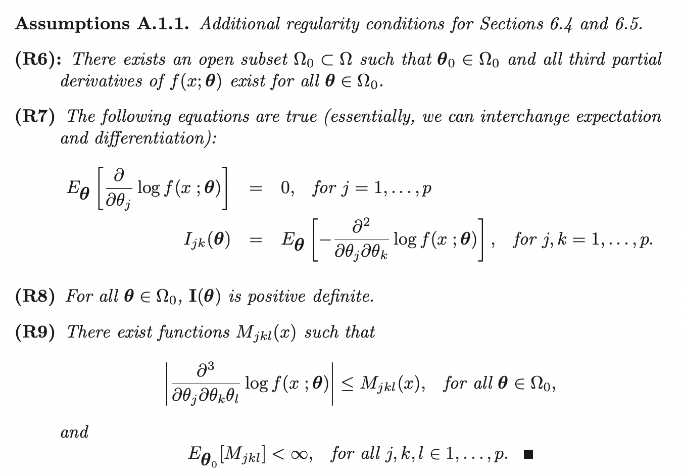
Fisher Information

The Fisher information in the scalar case is the variance of the random variable (the mean is 0):

\[E[(\frac{\partial \log f(X;\theta)}{\partial \theta})^2]\]

It measures the amount of information the random variable \(X\) carries about an unknown parameter \(\theta\).

In multivariate case, the variance becomes variance covariance matrix of \(\nabla_{\boldsymbol{\theta}} \log f_X(X;\boldsymbol{\theta})\):

\[I(\boldsymbol{\theta})_{j, k} = cov(\frac{\partial \log f_X(X;\boldsymbol{\theta})}{\partial \theta_j}, \frac{\partial \log f_X(X;\boldsymbol{\theta})}{\partial \theta_k})\]

By assumption, we can swap integral and derivative, thus we have:

\[\begin{aligned} 0 &= \int_{x} \frac{\partial f(x; \boldsymbol{\theta})}{\partial \theta_j} dx \\ &= \int_{x} \frac{\partial \log f(x; \boldsymbol{\theta})}{\partial \theta_j} f(x; \boldsymbol{\theta})dx\\ &= E[\frac{\partial \log f(X; \boldsymbol{\theta})}{\partial \theta_j}] \end{aligned}\]

If we take the partial derivative w.r.t \(\theta_k\), after multiplication rule, we have:

\[0 = \int_{x} \frac{\partial^2 \log f(x; \boldsymbol{\theta})}{\partial \theta_j\theta_k} \log f(x; \boldsymbol{\theta})dx + \int_x \frac{\partial \log f(x; \boldsymbol{\theta})}{\partial \theta_j}\frac{\partial \log f(x; \boldsymbol{\theta})}{\partial \theta_k} \log f(x; \boldsymbol{\theta})dx\] \[\implies -E[\frac{\partial^2 \log f(X; \boldsymbol{\theta})}{\partial \theta_j\theta_k}] = E[\frac{\partial \log f(X; \boldsymbol{\theta})}{\partial \theta_j}\frac{\partial \log f(X; \boldsymbol{\theta})}{\partial \theta_k}]\]

Thus, the fisher information matrix can be written as:

\[\begin{aligned} cov(\frac{\partial \log f_X(X;\boldsymbol{\theta})}{\partial \theta_j}, \frac{\partial \log f_X(X;\boldsymbol{\theta})}{\partial \theta_k}) &= E[\frac{\partial \log f_X(X;\boldsymbol{\theta})}{\partial \theta_j}\frac{\partial \log f_X(X;\boldsymbol{\theta})}{\partial \theta_k}] - E[\frac{\partial \log f(x; \boldsymbol{\theta})}{\partial \theta_j}]E[\frac{\partial \log f(x; \boldsymbol{\theta})}{\partial \theta_k}]\\ &= E[\frac{\partial \log f_X(X;\boldsymbol{\theta})}{\partial \theta_j}\frac{\partial \log f_X(X;\boldsymbol{\theta})}{\partial \theta_k}]\\ \implies I(\boldsymbol{\theta})_{j, k} &= E[\frac{\partial \log f_X(X;\boldsymbol{\theta})}{\partial \theta_j}\frac{\partial \log f_X(X;\boldsymbol{\theta})}{\partial \theta_k}]\\ &= -E[\frac{\partial^2 \log f(X; \boldsymbol{\theta})}{\partial \theta_j\theta_k}] \end{aligned}\]

By replacing \(f_X(X; \boldsymbol{\theta})\) by the likelihood function \(L(\boldsymbol{\theta}; \mathbf{X})\), we have:

\[Cov(\sum^{n}_{i=1}\nabla_{\boldsymbol{\theta}} f_X(X; \boldsymbol{\theta})) = nI(\boldsymbol{\theta})\]

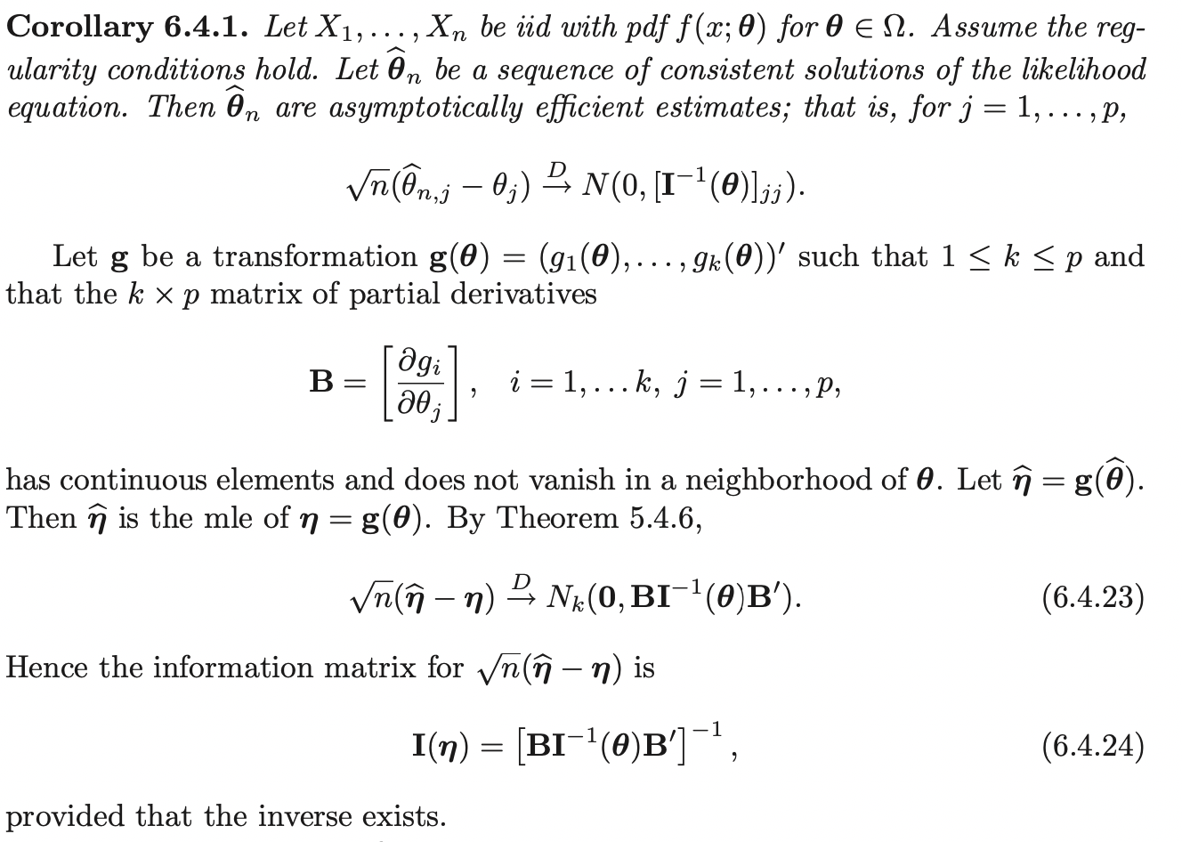
If \(Y_j = u_j (\mathbf{X})\) is an unbiased estimator of \(\theta_j\), then ti can be shown that:

\[Var(Y_j) \leq \frac{1}{n} [I^{-1}(\boldsymbol{\theta})_{jj}]\]

Then the estimator \(Y_j\) is called efficient.

Sufficiency

Measures of Quality of Estimators

Bayesian Statistics

Maximum A Posterior Estimation

MLE is not the only way to estimate the parameters. The paradigm of MAP is that we should choose the value for our parameters that is the most likely given the data, that is:

\[\hat{\theta} = \underset{\theta}{\arg\max}\; P(\theta| D)\]

If we have random sample \(X_1, ...., X_n\) that follows some discrete distribution \(P(X)\), then:

\[\begin{aligned} \hat{\theta} &= \underset{\theta}{\arg\max}\; p_X(\theta| X_1, ...., X_n)\\ &= \underset{\theta}{\arg\max}\; \frac{p_X(X_1, ...., X_n | \theta) P(\theta)}{p_X(X_1, ..., X_n)}\\ &= \underset{\theta}{\arg\max}\; p_X(X_1, ...., X_n | \theta) P(\theta)\\ &= \underset{\theta}{\arg\max}\; \prod^{N}_{i=1} p_X(X_i | \theta) P(\theta) \end{aligned}\]

Which is similar to maximum likelihood but with extra prior term \(P(\theta)\). Comparing to MAP, MLE chooses the value of parameters that makes the data most likely.

Ref

https://online.stat.psu.edu/stat415/lesson/1/1.2

https://web.stanford.edu/class/archive/cs/cs109/cs109.1192/reader/11%20Parameter%20Estimation.pdf