Backpropagation in CNN
Backpropagation In Convolutional Neural Networks
Cross Correlation
Given an input image \(I\) and a filter \(K\) of dimensions \(k_1 \times k_2\), then the cross correlation operation is defined as:
\[(I \otimes K)_{ij} = \sum^{k_2 - 1}_{m=0}\sum^{k_1 - 1}_{n=0} I(i + m, j + n)K(m, n)\]
Convolution
\[(I * K)^{d}_{ij} = \sum^{k_2 - 1}_{m=0}\sum^{k_1 - 1}_{n=0} I(i - m, j - n)K(m, n)\]
which is equivalent to cross correlation with flipped kernel (i.e flipped 180 degree)
\[(I * K)_{ij} = \sum^{k_2 - 1}_{m=0}\sum^{k_1 - 1}_{n=0} I(i + m, j + n) \text{ rot}_{180}(K(m, n))\]
CNNs
a Convolution layer consists of:
- An input map \(I \in \mathbb{R}^{H \times W \times C}\) with height \(H\), width \(W\), channels \(H\).
- A bank of \(D\) filters \(K \in \mathbb{R}^{k_1 \times k_2 \times D}\).
- Bias \(b \in \mathbb{R}^{D}\) (one for each filter).
- An activation function \(f\) apply element-wise.
In general, the forward output of applying filter \(d\) on the input map is:
\[(I * K^d)_{ij} = \sum^{k_2 - 1}_{m=0}\sum^{k_1 - 1}_{n=0} \sum^{C}_{n=1}I(i + m, j + n, c) \cdot \text{ rot}_{180}(K^d(m, n, c)) + b\]
However, in CNN, we do not care about the arrangement of filters (i.e whether it is flipped or not), because the weights are going to be learned regardless of the arrangement of the filters. Thus, we can safely ignore the flip and treat the convolution operation as cross correlation:
\[(I * K^d)_{ij} = \sum^{k_2 - 1}_{m=0}\sum^{k_1 - 1}_{n=0} \sum^{C}_{n=1}I(i + m, j + n, c) \cdot K^d(m, n, c) + b\]
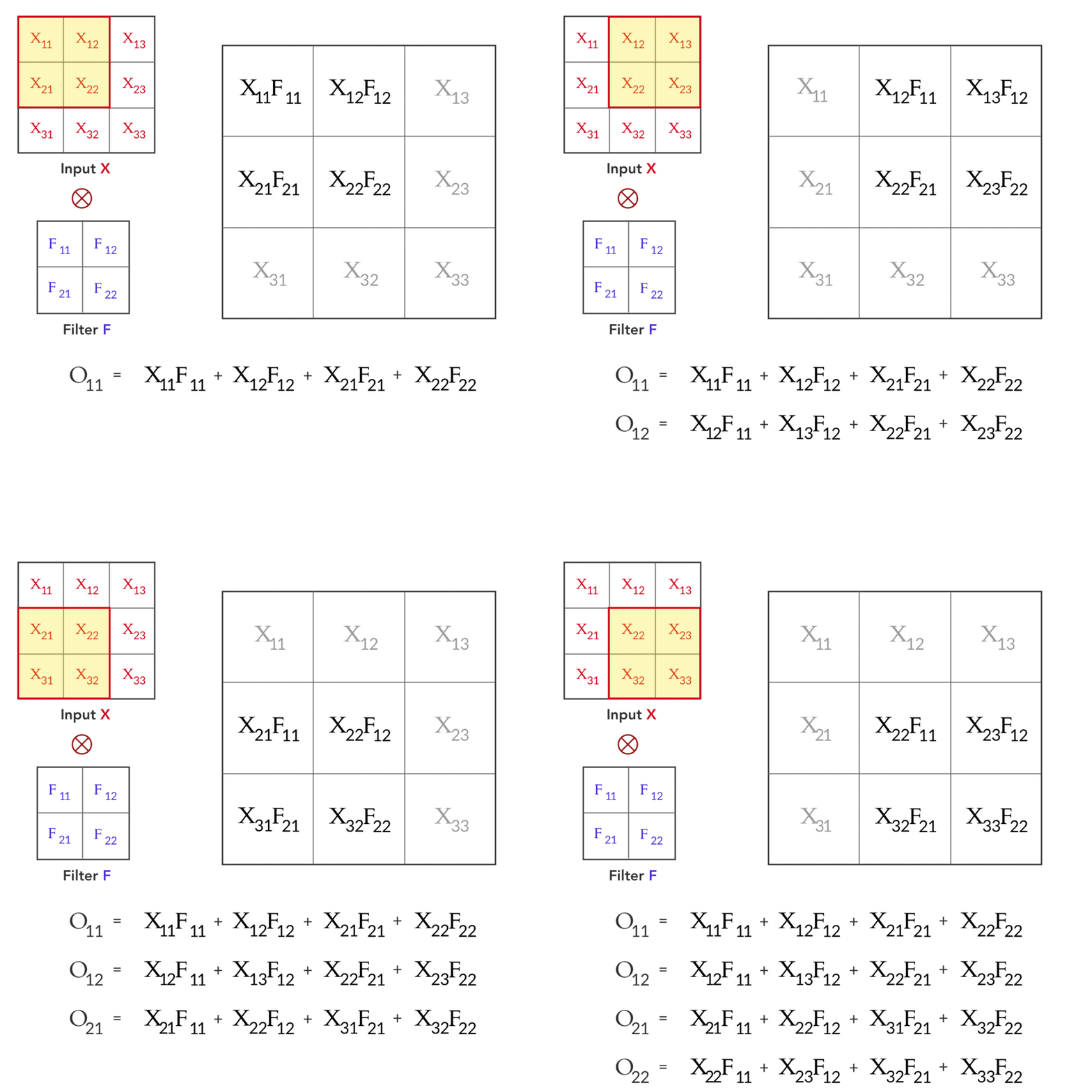
For the simplicity, we focus on \(2d\) case first (i.e we focus on gray scale image with \(C = 1\)) and only one filter:
\[(I * K)_{ij} = \sum^{k_2 - 1}_{m=0}\sum^{k_1 - 1}_{n=0} I(i + m, j + n)K(m, n)\]
Notations
- \(l\) is the \(l\)th layer, where \(l = 1\) is the first layer, \(L\) is the last layer.
- Input \(\mathbf{x}\) has dimension \(H \times W\).
- The filter weight at each layer is denoted as \(w^l_{m, n}, \; 0 \leq m < k^l_1, \; 0 \leq n < k^l_2\)
- The convolved input at each layer is denoted as \(y^{l}_{ij}\): \[y^{l}_{i, j} = \sum^{k^l_2 - 1}_{m=0}\sum^{k^l_1 - 1}_{n=0} w^{l}_{m, n} x^{l - 1}_{i+m, j+n} + b^l\]
- The output of each convolution layer after applying the activation function is denoted as: \[x^{l}_{ij} = f(y^{l}_{i, j})\]
Forward Pass
The forward pass is essential characterized above:

Backward Pass
Let the mean square loss be defined as:
\[L = \frac{1}{N} \sum^{N}_{i=1} (t_i - y^L_i)^2\]
Where \(y^L_i\) is the prediction from the final layer and \(t_i\) is the target value.
In backward propagation, we are seeking to compute the gradient of loss w.r.t the weights \(\frac{\partial L}{\partial w^{l}_{m, n}}\) for each layer, and the gradient w.r.t the output map to each layer \(\frac{\partial L}{\partial y^l_{i, j}}\).
Gradient of the Weights
Since, the output map \(\mathbf{y}^l\) will have dimension \(H^{l} = H^{l - 1} - k^l_{1} + 1\), \(W^{l} = W^{l - 1} - k^{l}_2 + 1\) (\(\mathbf{y}^{l}\) is reshaped to be a \(H^{l} W^{l} \times 1\) vector)
\[\begin{aligned} \frac{\partial L}{\partial w^{l}_{m^{\prime}, n^{\prime}}} &= \frac{\partial L}{\partial \mathbf{y}^l} \frac{\partial \mathbf{y}^{l}}{\partial w^{l}_{m^{\prime}, n^{\prime}}}\\ &= \sum^{H^{l} - 1}_{i=0} \sum^{W^{l} - 1}_{j=0}\frac{\partial L}{\partial y^l_{i, j}}\frac{\partial y_{i, j}^{l}}{\partial w^{l}_{m^{\prime}, n^{\prime}}}\\ \end{aligned}\]By expanding \(\frac{\partial y_{i, j}^{l}}{\partial w^{l}_{m^{\prime}, n^{\prime}}}\) we have:
\[\begin{aligned} \frac{\partial y_{i, j}^{l}}{\partial w^{l}_{m^{\prime}, n^{\prime}}} &= \frac{\partial}{\partial w^{l}_{m^{\prime}, n^{\prime}}}\sum^{k^l_2 - 1}_{m=0}\sum^{k^l_1 - 1}_{n=0} w^{l}_{m, n} x^{l - 1}_{i+m, j+n} + b^l\\ &= x^{l - 1}_{i + m^{\prime}, j + n^{\prime}} \end{aligned}\]By substituting the above result back to the previous gradient equation we have:
\[\frac{\partial L}{\partial w^{l}_{m^{\prime}, n^{\prime}}} = \sum^{H^{l} - 1}_{i=0} \sum^{W^{l} - 1}_{j=0}\frac{\partial L}{\partial y^l_{i, j}} x^{l - 1}_{i + m^{\prime}, j + n^{\prime}}\]
We can see that this is the convolution (cross correlation) of gradient of activations on the input feature map:
\[\frac{\partial L}{\partial w^{l}_{m^{\prime}, n^{\prime}}} = (X^{l - 1} \otimes \frac{\partial L}{\partial \mathbf{y}^l})_{m^{\prime}, n^{\prime}}\]
Where \(\frac{\partial L}{\partial \mathbf{y}^l}\) is reshaped to a \(H^l \times W^l\) matrix.
Gradients of the Inputs
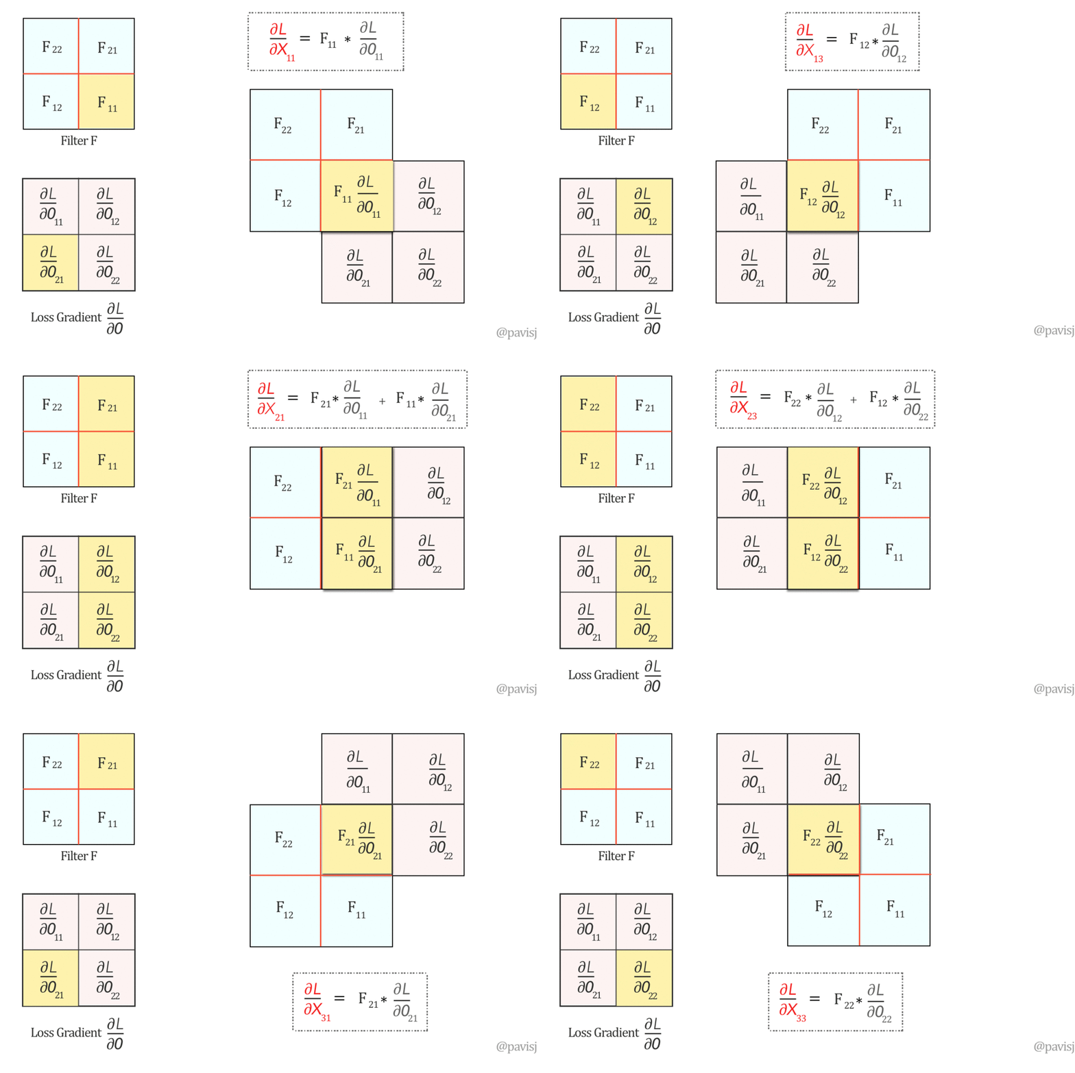
Recall that, \(\mathbf{x}^l = f(\mathbf{y}^l)\), so they have same dimensions.
\[\begin{aligned} \frac{\partial L}{\partial y^l_{i, j}} &= \frac{\partial L}{\partial \mathbf{x}^l} \frac{\partial \mathbf{x}^l}{\partial y_{i, j}^l}\\ &= \sum^{H^{l} - 1}_{i=0} \sum^{W^{l} - 1}_{j=0} \frac{\partial L}{\partial x^l_{i, j}} f^{\prime} (y^l_{i, j})\\ \\ \frac{\partial L}{\partial x^l_{i^{\prime}, j^{\prime}}} &= \frac{\partial L}{\partial \mathbf{y}^{l + 1}} \frac{\partial \mathbf{y}^{l + 1}}{\partial x^l_{i^{\prime}, j^{\prime}}}\\ &= \sum^{H^{l + 1} - 1}_{i=0} \sum^{W^{l + 1} - 1}_{j=0} \frac{\partial L}{\partial y^{l + 1}_{i^{\prime} - m, j^{\prime} - n}} w^{l + 1}_{m, n} \end{aligned}\]This is exactly as the full convolution (or correlation with flipped kernel, notice here, we have to flip the kernel):
\[\frac{\partial L}{\partial x^l_{i^{\prime}, j^{\prime}}} = (\frac{\partial L}{\partial \mathbf{y}^{l + 1}} * W^{l + 1} )_{i^{\prime}, j^{\prime}}\]
Where \(W^{l + 1}\) and \(\frac{\partial L}{\partial \mathbf{y}^{l + 1}}\) are reshaped into matrices.

Implementation
1 | import numpy as np |
Ref
https://www.jefkine.com/general/2016/09/05/backpropagation-in-convolutional-neural-networks/
https://medium.com/@pavisj/convolutions-and-backpropagations-46026a8f5d2c