Adaboost

AdaBoost (Discrete)

Consider a two-class problem, with the output variable coded as \(Y \in \{-1, 1\}\). Given a vector of input variables \(\mathbf{X}\), a classifier \(G(\mathbf{X})\) produces a prediction taking one of the two values \(\{-1, 1\}\).

Suppose we have samples \(D = \{(\mathbf{x}_1, y_1), ...., (\mathbf{x}_N, y_N); \; \mathbf{x} \in \mathbb{R}^d\}\). The error rate (misclassification) on the training sample is defined as:

\[\bar{err} = \frac{1}{N} \sum^{N}_{i=1} I[y_i \neq G(\mathbf{x}_i)]\]

The expected error rate is defined as:

\[E_{X, Y} [I[Y \neq G(\mathbf{X})]]\]

A weak classifier is one whose error rate is only slightly better than random guessing. The purpose of boosting is to sequentially apply the weak classification algorithm to repeatedly modified versions of the data, thereby producing a sequence of weak classifiers \(G_{m} (\mathbf{x}), \; m = 1, ...., M\)

The predictions from all of them are then combined through a weighted majority vote to produce the final prediction:

\[G(x) = sign (\sum^{M}_{m=1} \alpha_m G_m (\mathbf{x}))\]

Here, \(\alpha_1, ...., \alpha_M\) are parameters that weight the contribution of each corresponding classifier \(G(\mathbf{x})\) and they are learned by the algorithm. They are here to give higher influence to the more accurate classifiers in the sequence.

The data modifications at each boosting step consist of applying weights \(w_1, ...., w_N\) to each of the training observations \((\mathbf{x}_i, y_i), \; i=1, ....., N\):

1. Initially all of the weights are set to \(w_i = \frac{1}{N}\), so the first step simply trains the classifier on the data in usual manner.
2. For each successive iteration \(m = 2, 3, .... , M\), the observation weights are individually modified:
   • Observations that were misclassified by the classifier \(G_{m-1} (\mathbf{x})\) induced at the previous step have their weights increased.
   • Observations that were classified correctly by the previous classifier have their weights decreased.
3. Then the classification algorithm is reapplied to the weighted observations

So misclassified samples have their weights increased so that each successive classifier is thereby forced to concentrate on those samples.

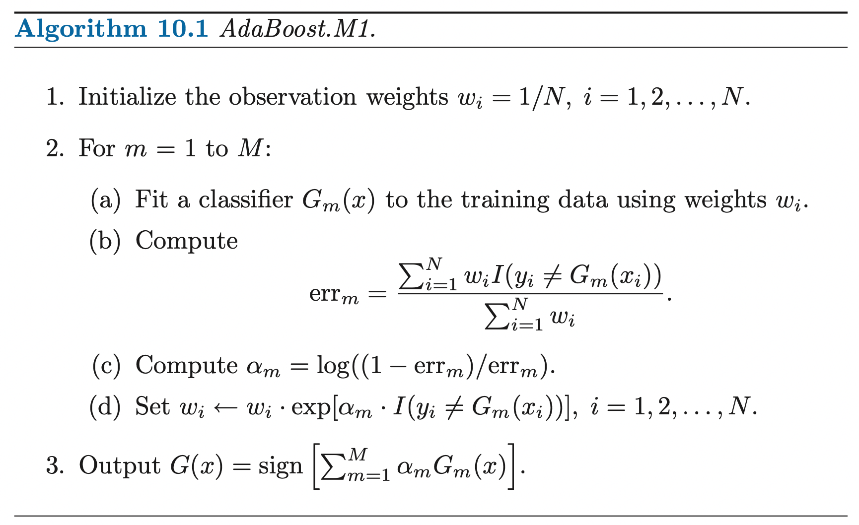
At each iteration \(m\):

1. A normalized weighted error rate (high penalty for misclassifying high weight samples)\(err_m\) is calculated.
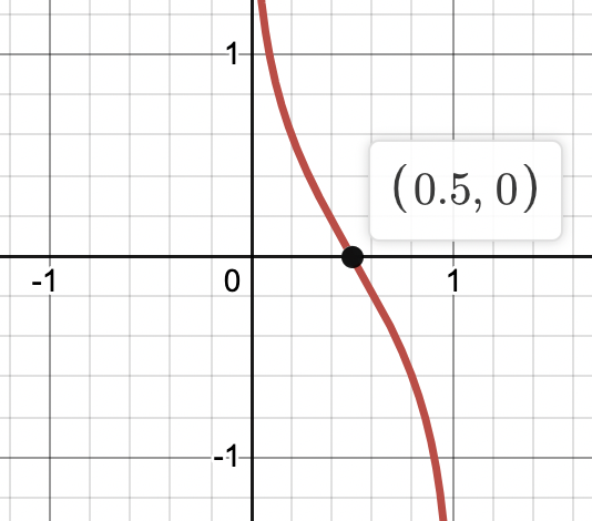
2. The error rate is transformed by \(\log (\frac{1 - error_m}{error_m})\):
   • This function goes to positive infinity as \(error_m\) goes to 0
   • This function goes to negative infinity as \(error_m\) goes to 1 (we should just predict class inversely)
   • This function is 0 when error rate is 0.5
3. The new weight update:
   • If correctly classified, then we simply keep the original weight for the sample (It will be smaller because we are weighting it by sum of error rate in the next classifier).
   • If incorrectly classified:
     • If error rate is small, then \(\alpha\) is positively large so each misclassified sample's weight is increased
     • If error rate is high, then \(\alpha\) goes to negative infinity, so each misclassified sample's weight is decreased because this sample is correctly classified inversely so we decrease its weight.
     • If error rate is 0.5, then \(\alpha\) is 0, so each misclassified sample's weight is maintained

Boosting Fits an Additive Model

Boosting is a way of fitting an additive expansion in a set of elementary basis functions. Here the basis functions are the individual classifiers \(G_m(\mathbf{x}) \in \{-1, 1\}\). More generally, basis function expansions take the form:

\[f(\mathbf{x}) = \sum^{M}_{m=1} \beta_m b(\mathbf{x}; \boldsymbol{\gamma}_m)\]

Where \(\beta_m, \; m=1, 2, ...., M\) are the expansion coefficients, and \(b(\mathbf{x}; \gamma) \in \mathbb{R}\) are usually simple functions of multivariate argument \(\mathbf{x}\) characterized by a set of parameters \(\{\boldsymbol{\gamma}_1, ...., \boldsymbol{\gamma}_M\}\).

Typically these models are fit and the parameters are found by minimizing a loss function averaged over the training data:

\[\min_{ \{\beta_m, \boldsymbol{\gamma}_m\}^{M}_1 }\sum^{N}_{i=1} L(y_i, \sum^{M}_{m=1} \beta_m b(\mathbf{x}_i; \boldsymbol{\gamma}_m))\]

Forward Stagewise Additive Modeling

How to solve the above optimization problem? We can use forward stagewise modeling (greedy) to approximate the solution to above equation by sequentially adding new basis functions to the expansion without adjusting the parameters and coefficients of those that have already been added.

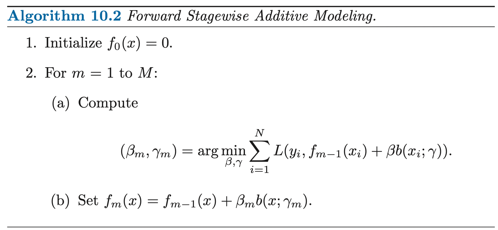
The loss function of optimization problem at each step \(m\) can be rewritten as:

\[L(y_i, f_m(\mathbf{x}_i)) = L(y_i, f_{m-1} (\mathbf{x}_i) + \beta b(\mathbf{x}_i; \boldsymbol{\gamma}))\]

Using the square loss, we have:

\[L(y_i, f_m(\mathbf{x}_i)) = (y_i - f_{m-1} (\mathbf{x}_i) - \beta b(\mathbf{x}_i; \boldsymbol{\gamma}))^2\]

\[\implies L(y_i, f_m(\mathbf{x}_i)) = (\epsilon_{im-1} - \beta b(\mathbf{x}_i; \boldsymbol{\gamma}))^2\]

This implies that we are fitting a basis function at each step to minimizing the residual from the current model \(f_{m-1} (\mathbf{x})\).

AdaBoost as Forward Stagewise Additive Modeling

Let the loss function be the exponential function:

\[L(y_i, f(\mathbf{x}_i)) = e^{-y_i f(\mathbf{x}_i)}\]

For adaboost, the basis functions are individual weak classifier \(G_m(x) \in \{-1, 1\}\). Using the exponential loss for additive stagewise modeling, we must minimize the objective:

\[(\beta_m, G_m) = \underset{\beta, G}{\arg\min} \sum^{N}_{i=1} e^{-y_i(f_{m-1} (\mathbf{x}_i) + \beta G(\mathbf{x}_i))}\]

Let \(w^{(m)}_i = e^{-y_i \mathbf{x}_i}\), then the above optimization can be expressed as:

\[(\beta_m, G_m) = \underset{\beta, G}{\arg\min} \sum^{N}_{i=1} w^{(m)}_i e^{-y_i\beta G(\mathbf{x}_i)}\]

Since, \(w^{(m)}_i\) does not depend on \(\beta, G(\mathbf{x})\), so it is just some constant and can be regard it as weight. Since this weight depends on previous prediction and current label, it is changing at each iteration \(m\).

Solve for \(\beta\)

In order to solve for \(\beta\), we can rewrite the objective as:

\[\begin{aligned} \sum^{N}_{i=1} w^{(m)}_i e^{-y_i\beta G(\mathbf{x}_i)} &= \sum^{N}_{i=1} w^{(m)}_i e^{-\beta} I[y_i = G(\mathbf{x}_i)] + w^{(m)}_i e^{\beta} I[y_i \neq G(\mathbf{x}_i)] \\ &= \sum^{N}_{i=1} w^{(m)}_i e^{-\beta} (1 - I[y_i \neq G(\mathbf{x}_i)]) + w^{(m)}_i e^{\beta} I[y_i \neq G(\mathbf{x}_i)]\\ &= (e^{\beta} - e^{-\beta})\sum^{N}_{i=1} w^{m}_i I[y_i \neq G(\mathbf{x}_i)] + e^{-\beta} \sum^{N}_{i=1} w^{(m)}_i \end{aligned}\]

by taking the partial derivative w.r.t \(\beta\) and set it to 0:

\[\implies(e^\beta + e^{-\beta}) \sum_{i=1}^{N} w_i^{(m)}I(y_i \neq G(\mathbf{x}_i)) - e^{-\beta} \sum_{i=1}^{N} w_i^{(m)} = 0\]

\[\implies \frac{e^\beta + e^{-\beta}}{e^{-\beta}} = \frac{\sum_{i=1}^{N} w_i^{(m)}}{\sum_{i=1}^{N} w_i^{(m)}I(y_i \neq G(\mathbf{x}_i))}\]

\[\implies \frac{e^\beta}{e^{-\beta}} = \frac{\sum_{i=1}^{N} w_i^{(m)}}{\sum_{i=1}^{N} w_i^{(m)}I(y_i \neq G(\mathbf{x}_i))} - 1\]

\[\implies 2\beta = \log(\frac{1}{error_m} - 1)\]

\[\implies \beta_m = \frac{1}{2} \log (\frac{1 - error_m}{error_m})\]

Where \(error_m = \frac{\sum_{i=1}^{N} w_i^{(m)}I(y_i \neq G(\mathbf{x}_i))}{\sum_{i=1}^{N} w_i^{(m)}}\)

That is, for any classifier \(G\):

• \(\beta_m > 0\), if \(error_m < 0.5\)
• \(\beta_m < 0\), if \(error_m > 0.5\)

Solve for \(G\)

We want our basis function (weak classifier) to have better misclassification rate than random classifier, so we want \(error_m < 0.5\) which implies that we want \(\beta > 0\). Thus, for any value \(\beta > 0\), we can see that if we let \(G(\mathbf{x}_i) = y_i\) for all samples, we have minimum objective. Thus, we can transform the minimization problem to minimize the error rate:

\[\begin{aligned} G_m = \underset{G}{\arg\min} \sum^{N}_{i=1} w^{(m)}_i I[y_i \neq G(\mathbf{x}_i)] \end{aligned}\]

By substitute \(G_m\) back to the solution of \(\beta\), we have:

\[\beta_m = \frac{1}{2} \log (\frac{1 - error_m}{error_m})\]

Where \(error_m = \frac{\sum_{i=1}^{N} w_i^{(m)}I(y_i \neq G_m(\mathbf{x}_i))}{\sum_{i=1}^{N} w_i^{(m)}}\)

The approximation is then updated:

\[f_m (\mathbf{x}_i) = f_{m-1} (\mathbf{x}_i) + \beta_m G_m (\mathbf{x}_i)\]

Which causes the weights for the next iteration to be:

\[\begin{aligned} w^{(m + 1)}_i &= e^{-y_i f_{m} (\mathbf{x}_i)}\\ &= e^{-y_i (f_{m - 1} (\mathbf{x}_i) + \beta_m G_m (\mathbf{x}_i))}\\ &= e^{-y_i f_{m-1}(\mathbf{x}_i)} e^{-y_i \beta_m G_m (\mathbf{x}_i)}\\ &= w^{(m)}_{i} e^{-y_i \beta_m G_m (\mathbf{x}_i)} \end{aligned}\]

Notice here, \(-y_i G_m (x_i) = 2 I[y_i \neq G_m (\mathbf{x}_i)] - 1\):

\[\implies w^{(m + 1)}_i = w^{(m)}_{i} e^{\alpha_m I[y_i \neq G_m(\mathbf{x}_i)]} e^{-\beta_m }\]

Where, \(\alpha_m = 2 \beta_m\) is the \(\alpha_m\) in Adaboost algorithm, and \(e^{-\beta_m}\) has no effect on weights because it is just a constant multiplying every sample.

Conclusion

Thus, we can think of Adaboost algorithm as stagewise additive modeling with basis function as a weak classifier (Minimizing the misclassification rate to have slightly better misclassification rate than random classifier) and exponential loss function.

Ref

ESLII Chapter 10