GBDT

Gradient Boosting Decision Trees

Boosting Trees

Regression and classification trees partition the space of all joint predictor variable values into disjoint regions \(R_j, \; j=1, 2, ...., J\) as represented by the terminal nodes of the tree. A constant \(c_j\) is assigned to each such region and the prediction rule is:

\[\mathbf{x} \in R_j \implies f(\mathbf{x}) = c_j\]

Thus, a tree can be formally expressed as:

\[T(\mathbf{x}; \boldsymbol{\theta}) = \sum^{J}_{j=1} c_j I[\mathbf{x} \in R_j]\]

with parameters \(\theta = \{R_j, c_j\}^J_1\). The parameters are found by iteratively solving minimizing problem:

1. Given \(R_j\), we solve \(\hat{c}_j\) by simply taking the average or majority class.
2. \(R_j\) is found by iterating over all possible pairs of feature and splitting point.

The boosted tree model is a sum of such trees induced in a forward stagewise manner:

\[f_M (\mathbf{x}) = \sum^{M}_{m=1} T(\mathbf{x}; \; \boldsymbol{\theta}_m)\]

At each step, one must solve:

\[\hat{\boldsymbol{\theta}}_m = \underset{\boldsymbol{\theta}_m}{\arg\min} \sum^{N}_{i=1} L(y_i, f_{m-1} (\mathbf{x}_i) + T(\mathbf{x}_i; \; \boldsymbol{\theta}_m))\]

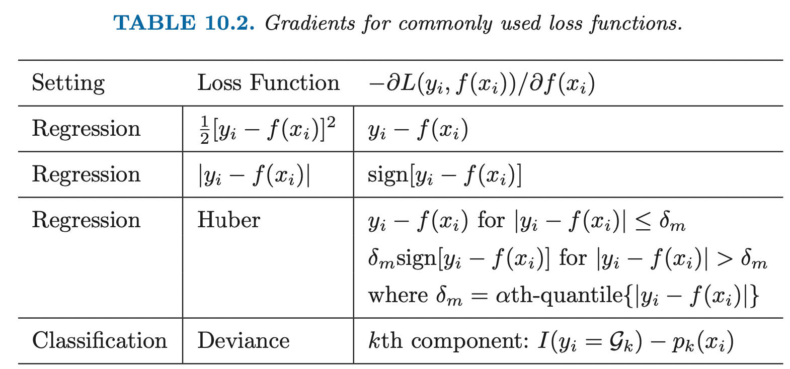
Gradient Boosting

In general, it is hard to directly take partial derivatives w.r.t the tree's parameters, thus, we take partial derivatives of tree predictions \(f(\mathbf{x}_i)\).

Fast approximate algorithms for solving the above problem with any differentiable loss criterion can be derived by analogy to numerical optimization. We first start with general case. The loss in using \(\mathbf{f}\) to predict \(y\) on the training data is:

\[L(\mathbf{f}) = \sum^{N}_{i=1} L(y_i, f(\mathbf{x}_i))\]

The goal is to minimize \(L(\mathbf{x}_i)\) w.r.t \(f\), where here \(f(\mathbf{x})\) is constrained to be a sum of trees \(f_M (\mathbf{x})\).

We first start with general case where \(f\) can be any parameters or numbers. In this case, we have \(N\) samples, thus, \(\mathbf{f} = \{f(\mathbf{x}_1), ...., f(\mathbf{x}_N)\} \in \mathbb{R}^N\).

Then, the gradient of objective w.r.t \(\mathbf{f} = \mathbf{f}_{m-1}\) which is the current model is:

\[\mathbf{g}_m = \nabla_{\mathbf{f}} L(\mathbf{f}) = \; <\frac{\partial L(\mathbf{f})}{\partial f(\mathbf{x}_1)}, ...., \frac{\partial L(\mathbf{f})}{\partial f(\mathbf{x}_N)}>\]

Then this gradient points at the direction of steepest increase, it tells us how we can change our current predictions to increase our loss. Since we want to minimize the objective, we would like to adjust our current predictions to the direction of steepest decrease:

\[\mathbf{h}_m = - \rho_m \mathbf{g}_m\]

Where \(\rho_m\) is the step size for current model and it is minimizer of:

\[\rho_m = \underset{\rho}{\arg\min} \; L(\mathbf{f}_{m-1} - \rho\mathbf{g}_m)\]

The current solution is then updated as

\[\mathbf{f}_{m} = f_{m-1} - \rho_m\mathbf{g}_m\]

If fitting the training data (minimizing the loss) is our ultimate goal, then the above update rule can solve our problem by adding the negative gradient at each iteration. However, our ultimate goal is to generalize to new data, copying and pasting training data exactly is not what we want. One possible solution is to learn the update \(- \rho_m\mathbf{g}_m\) by fitting a simple decision tree:

\[\hat{\boldsymbol{\theta}}_m = \underset{\boldsymbol{\theta}}{\arg\min} \sum^{N}_{i=1} (-g_{im} - T(x_i; \; \boldsymbol{\theta}))^2\]

That is, we fit a regression tree \(T\) to the negative gradient values.

Algorithm

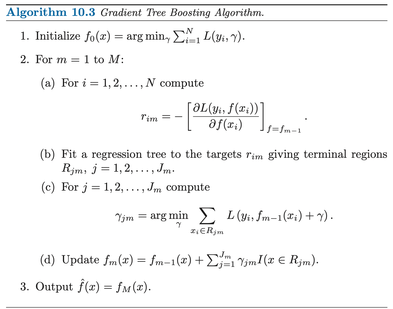
1. We first start by a constant model (model that predict constants) which is a single terminal node tree.
2. For all samples new targets are generated to be the negative gradient of the loss function w.r.t the current model prediction \(\mathbf{f}_{m-1}\).
3. Fit a regression tree to minimize the MSE between new target (negative gradient) and current prediction.

Discussions

Regularization

For numbers of gradient boosting rounds \(M\), the loss can be made arbitrarily small. However, fitting the data too well can lead to overfitting which degrades the risk on future predictions.

Shrinkage

Controlling the value of \(M\) is not the only possible regularization strategy, we can add penalty terms to the loss function that penalize large \(M\) or we can weight subsequent trees. The simplest implementation of shrinkage in the context of boosting is to scale the contribution of each tree by a factor of \(0 < v < 1\), when it is added to the current approximation:

\[f_m (\mathbf{x}) = f_{m-1}(\mathbf{x}) + v \sum^{J}_{j=1} c_{jm} I[\mathbf{x} \in R_{jm}]\]

The parameter \(v\) can be regarded as controlling the learning rate of the boosting procedure. Smaller values of \(v\) result in larger training error for the same number of iterations \(M\) but might have better generalization. Thus, both \(v\) and \(M\) control prediction risk on the training data. \(v\) and \(M\) tradeoff each other, therefore in practice, it is best to set \(v\) small and control \(M\) by early stopping.

Subsampling

We know that bootstrap averaging (bagging) improves the performance of a noisy classifier through averaging (reduce variance). We can exploit the same idea in gradient boosting.

At each iteration, we sample a fraction \(\eta\) of the training observations without replacement, and grow the next tree using that subsample. A typical value of \(\eta\) is 0.5, although for large sample size \(N\), we can have smaller \(\eta\).

Ref

https://www.ccs.neu.edu/home/vip/teach/MLcourse/4_boosting/slides/gradient_boosting.pdf