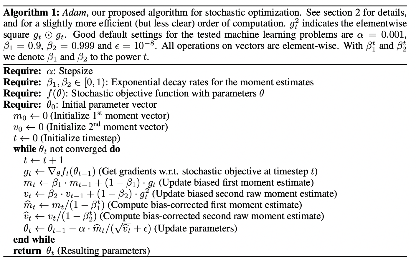
Adam

ADAM: A METHOD FOR STOCHASTIC OPTIMIZATION

Let \(F\) be a noisy objective function (stochastic function) defined as \(F(\boldsymbol{\theta})\) that is differentiable w.r.t \(\boldsymbol{\theta}\), we are interested in minimizing the expected value of this random function:

\[\min_{\boldsymbol{\theta}} E_{F}[F(\boldsymbol{\theta})]\]

Let \(F_1(\boldsymbol{\theta}), ...., F_{T} (\boldsymbol{\theta})\) be a random sample of \(F(\boldsymbol{\theta})\) and let \(f_1 (\boldsymbol{\theta}), ..., f_T(\boldsymbol{\theta})\) be the realization of random sample. This random sample can be forms of mini-batches of data which the distribution does not depend on the parameter \(\boldsymbol{\theta}\).

Then:

\[\nabla_{\boldsymbol{\theta}} E_F[F (\boldsymbol{\theta})] = E_F[\nabla_{\boldsymbol{\theta}} F (\boldsymbol{\theta})]\]

Given the individual sample gradient \(\nabla_{\boldsymbol{\theta}} f_1 (\boldsymbol{\theta}), ...., \nabla_{\boldsymbol{\theta}} f_T(\boldsymbol{\theta})\), one way to estimate the expectation of gradient, \(E_{F} [\nabla_{\boldsymbol{\theta}} F_t(\boldsymbol{\theta})]\), is to use stochastic approximation (similar to Momentum):

\[m_t \leftarrow \beta_1 {m}_{t} + (1 - \beta_1) \nabla_{\boldsymbol{\theta}} f_t(\boldsymbol{\theta})\]

Where \(m_t\) is the average up to sample \(t\), and \(\beta_1 \in [0, 1)\) is the decay rates.

At the same time, we can use SA to estimate the second moment of the gradient which is the un-centered variance (This is similar to RMSProp):

\[v_t \leftarrow \beta_2 {v}_{t} + (1 - \beta_2) \nabla_{\boldsymbol{\theta}} f_t(\boldsymbol{\theta})^2\]

However, these estimates are biased toward 0 if we initialize them to be 0 especially during initial timesteps and especially when the decay rates are small (\(\beta_1, \beta_2\) close to 1). Thus, we need to apply bias correction.

Initial Bias Correction

Let \(\mathbf{G} = \nabla_{\boldsymbol{\theta}} F\) be the gradient of the stochastic objective \(F\), we wish to estimate its second raw moment using SA of the squared gradient with decay rate \(\beta_2\). Let \(\mathbf{G}_1, ...., \mathbf{G}_T\) be random sample of \(\mathbf{G}\) that draws from the gradient distribution \(P(\mathbf{G})\). Suppose we initialize our SA procedure at \({v}_0 = 0\), then after \(t\) steps, we have:

\[v_1 = (1 - \beta_2) \mathbf{G}^2_1\]

\[v_2 = \beta_2(1 - \beta_2) \mathbf{G}^2_1 + (1 - \beta_2) \cdot \mathbf{G}^2_2 = \beta_2 (1 - \beta_2) (\mathbf{G}^2_1 + \mathbf{G}^2_2)\]

\[\implies {v}_t = (1 - \beta_2) \sum^{t}_{i=1} \beta^{t - i}_2 \mathbf{G}^2_{i}\]

Where \(\mathbf{G}^2 = \|\mathbf{G}\|^2_2\). We want the SA estimator to be unbiased estimator of second moment of gradient but we know that there is initialization bias (discrepancy) of SA estimator, we denote this discrepancy \(\eta\). Since additive discrepancy can be keep small by assigning less weight to history, we want two sides to be equal:

\[E_{\mathbf{G}} [\mathbf{G}^2] = E_\mathbf{G}[\mathbf{v}^2_t] + \eta = E_\mathbf{G} [(1 - \beta_2) \sum^{t}_{i=1} \beta_2^{t - i} \mathbf{G}^2_{i}] + \eta\]

However, since \(t < \infty\), we have a proportion bias:

\[\begin{aligned} E_\mathbf{G}[\mathbf{v}^2_t] + \eta &= E_{\mathbf{G}} [\mathbf{G}^2] (1 - \beta_2) \sum^{t}_{i=1} \beta_2^{t - i} + \eta\\ &= E_{\mathbf{G}} [\mathbf{G}^2] (1 - \beta_2) \sum^{t}_{i=1} \beta_2^{t}(\frac{1}{\beta_2})^i + \eta\\ &= E_{\mathbf{G}} [\mathbf{G}^2] (1 - \beta_2) \frac{1}{\beta_2} \sum^{t}_{i=0}\beta_2^{t}(\frac{1}{\beta_2})^i + \eta\\ &= E_{\mathbf{G}} [\mathbf{G}^2] (1 - \beta_2) \frac{1}{\beta_2} \beta_2^{t} \frac{\beta^t_2 - 1}{\beta^t_2} \frac{\beta_2}{\beta_2 - 1}+ \eta\\ &= E_{\mathbf{G}} [\mathbf{G}^2] \underbrace{(1 - \beta^t_2)}_{\text{This term we do not want}} + \eta \end{aligned}\]

Thus, we can apply a bias correction term on the estimator to correct for this proportion bias \(\frac{1}{1 - \beta^t_2}\).

The same correction \(\frac{1}{1 - \beta^t_1}\)is applied on first moment estimator of the gradient.

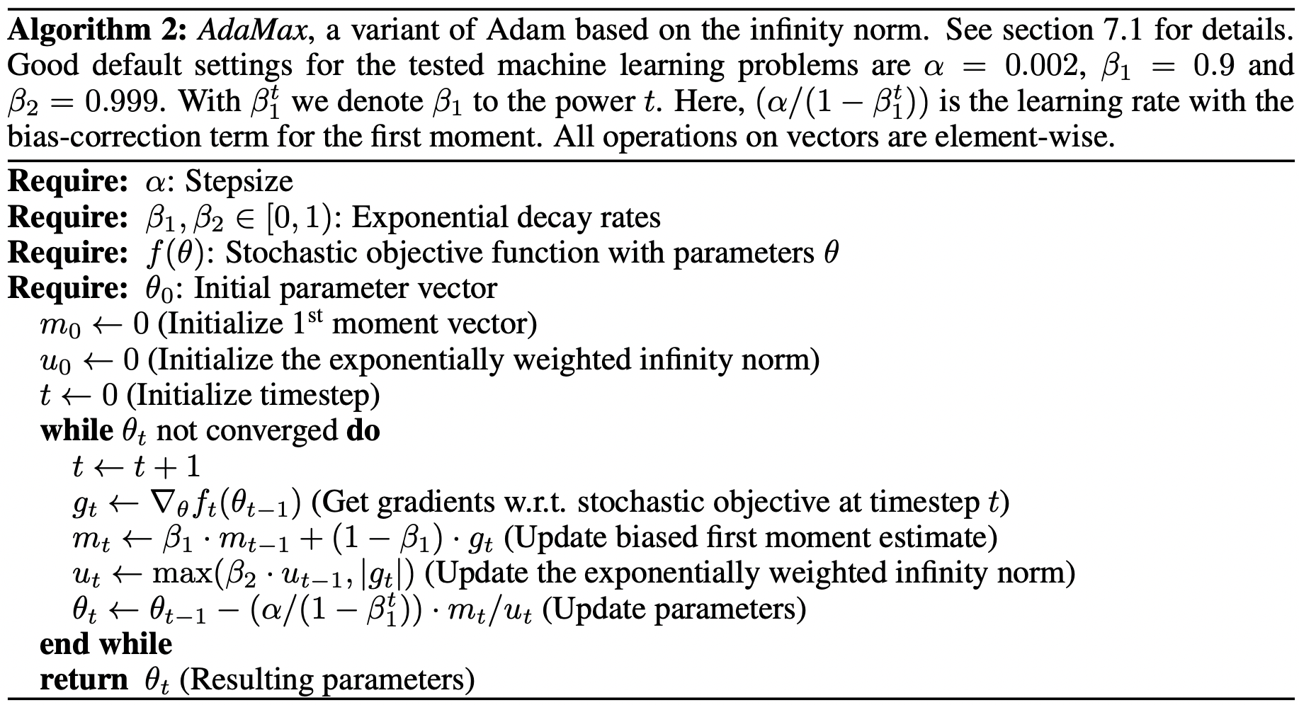
AdaMax

In Adam, the current average gradient estimate \(\hat{m}_t\) is scaled inversely to history proportional to the scaled \(L^2\) norm of their individual current and past gradients (i.e \(\frac{\alpha}{\sqrt{\hat{v}_t} + \epsilon}\)). We can generalize \(L^2\) norm to a \(L^\infty\) norm based update rule. This leads to a surprisingly simple and stable algorithm:

In case of \(L^p\) norm, \(\mathbf{v}_t\) is defined to be:

\[\begin{aligned} {v}_t &\leftarrow \beta^p_2 + {v}_t (1 - \beta^p_2) \|\mathbf{G}_i\|^p_p\\ &\leftarrow (1 - \beta_2^p) \sum^{t}_{i=1} \beta^{p(t - i)}_2 \|\mathbf{G}_i\|^p_p\\ \end{aligned}\]

Note define:

\[u_t = \lim_{p \rightarrow \infty} (v_t)^{\frac{1}{p}}\]

Then:

\[\begin{aligned} u_t &= \lim_{p \rightarrow \infty} (v_t)^{\frac{1}{p}}\\ &= \lim_{p \rightarrow \infty} ((1 - \beta_2^p) \sum^{t}_{i=1} \beta^{p(t - i)}_2 \|\mathbf{G}_i\|^p_p)^\frac{1}{p}\\ &= \lim_{p \rightarrow \infty} (1 - \beta_2^p)^\frac{1}{p} (\sum^{t}_{i=1} \beta^{p(t - i)}_2 \|\mathbf{G}_i\|^p_p)^\frac{1}{p}\\ &= \lim_{p \rightarrow \infty} (\sum^{t}_{i=1}(\beta^{(t - i)}_2 \|\mathbf{G}_i\|_p)^p)^\frac{1}{p}\\ &= \| \beta^{(t - i)}_2 \|\mathbf{G}_i\|_{\infty}\|_{\infty}\\ &= \max(\beta^{(t - 1)}_2 \|\mathbf{G}_1\|_{\infty}, .... , \|\mathbf{G}_t\|_{\infty}) \end{aligned}\]

Which corresponding to:

\[u_t \leftarrow \max(\beta_2 u_{t}, \|\mathbf{G}_t\|_{\infty})\]