RNN

Recurrent Neural Network

Introduction

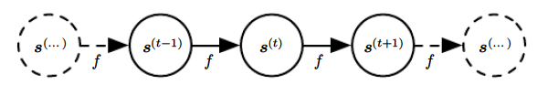
Consider the recurrent equation:

\[\mathbf{s}^{t} = f(\mathbf{s}^{t-1}; \; \boldsymbol{\theta})\]

For a finite time step \(\tau\), this equation can be unfolded by applying the definition \(\tau - 1\) times:

\[f(f(....f(\mathbf{s}^{1}; \; \boldsymbol{\theta}) ... ; \; \boldsymbol{\theta}) ; \; \boldsymbol{\theta})\]

Then, this expression can now be represented as a DAG because it no longer involves recurrence:

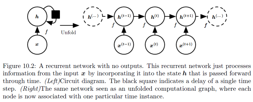
Notice here, the parameters \(\boldsymbol{\theta}\) are shared. The idea extends smoothly to:

\[\mathbf{s}^{t} = f(\mathbf{s}^{t-1}, \mathbf{x}^{t}; \; \boldsymbol{\theta})\]

We can see that now, \(s^{t}\) contains information about the whole past \(\mathbf{x}^1 , ....., \mathbf{x}^t\)

Many Recurrent Neural Networks use similar idea to express their hidden units:

\[\begin{aligned} \mathbf{h}^t &= f(\mathbf{h}^{t-1}, \mathbf{x}^t ; \; \boldsymbol{\theta})\\ &= g^t (\mathbf{x}^1 , ....., \mathbf{x}^t) \end{aligned}\]

Typically, RNN will have output layers to output predictions at given timesteps. When the recurrent network is trained to perform a task that requires predicting the future from the past, the network typically learns to use \(\mathbf{h}^t\) to give a lossy summary of past sequence up to time \(t\). The summary is lossy because we are mapping \(\mathbf{x}^1 , ....., \mathbf{x}^t\) to a fixed length \(\mathbf{h}^t\)

The unfolded structure has several advantages:

1. The learned model \(f\) is defined as transition from hidden units (input) \(h^{t - 1}\) to \(h^{t}\) (output) regardless the value of time \(t\). Thus, we can have one model for different lengths of sequences.
2. The parameters \(\boldsymbol{\theta}\) are shared.

Forward Pass

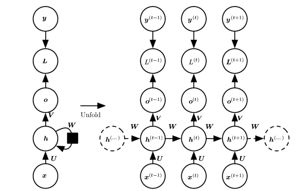
In formulas, the forward pass for same output and input length RNN with tanh non-linearity and probability as prediction can be described as starting from \(\mathbf{h}^0\):

\[\mathbf{a}^{t} = \mathbf{b} + W\mathbf{h}^{t-1} + U\mathbf{x}^{t}\] \[\mathbf{h}^t = \tanh (\mathbf{a}^t)\] \[\mathbf{o}^t = \mathbf{c} + V\mathbf{h}^t \] \[\hat{\mathbf{y}}^t = softmax(\mathbf{o}^t)\]

• \(W\) is the hidden to hidden weights that encodes information about past sequences.
• \(V\) is the hidden to output weights that is responsible for prediction using current hidden units.
• \(U\) is the input to hidden weights that is responsible for input parameterization.
• \(\mathbf{b}\) is the bias associated with \(W\)
• \(\mathbf{c}\) is the bias associated with \(V\)

Then the multi-class cross entropy loss of the sequence of \(\{(\mathbf{x}^{1}, \mathbf{y}^{1}) ,...., (\mathbf{x}^{\tau}, \mathbf{y}^{\tau})\}\) (\(\mathbf{y}\) is encoded as one hot vector) is just the sum of per timestep loss:

\[\begin{aligned} L(\{\mathbf{y}^{1}, ..., \mathbf{y}^{\tau}\}, \; \{\mathbf{\hat{y}}^{1}, ..., \mathbf{\hat{y}}^{\tau}\}) &= \sum^{\tau}_{i=1} L(\mathbf{y}^i, \; \mathbf{\hat{y}}^{i})\\ &= -\sum^{\tau}_{i=1} \sum_{k} y_k \log (\hat{y}^{i}_{k}) \end{aligned}\]

Where \(\hat{y}^{i}_{k}\) is the \(k\)th element of \(\mathbf{\hat{y}}^{i}\). Since we are using one-hot encoding, we can also write it as:

\[L(\{\mathbf{y}^{1}, ..., \mathbf{y}^{\tau}\}, \; \{\mathbf{\hat{y}}^{1}, ..., \mathbf{\hat{y}}^{\tau}\}) = -\sum^{\tau}_{i=1} \log (P_{\hat{Y}}(y^{i} | \{\mathbf{x}^{1}, ..., \mathbf{x}^{\tau}\}))\]

Where \(P_{\hat{Y}}(y^{i} | \{\mathbf{x}^{1}, ..., \mathbf{x}^{\tau}\})\) is the value of the target position (ie. the position of \(\mathbf{y}^{i}\) with 1) in \(\mathbf{\hat{y}}\).

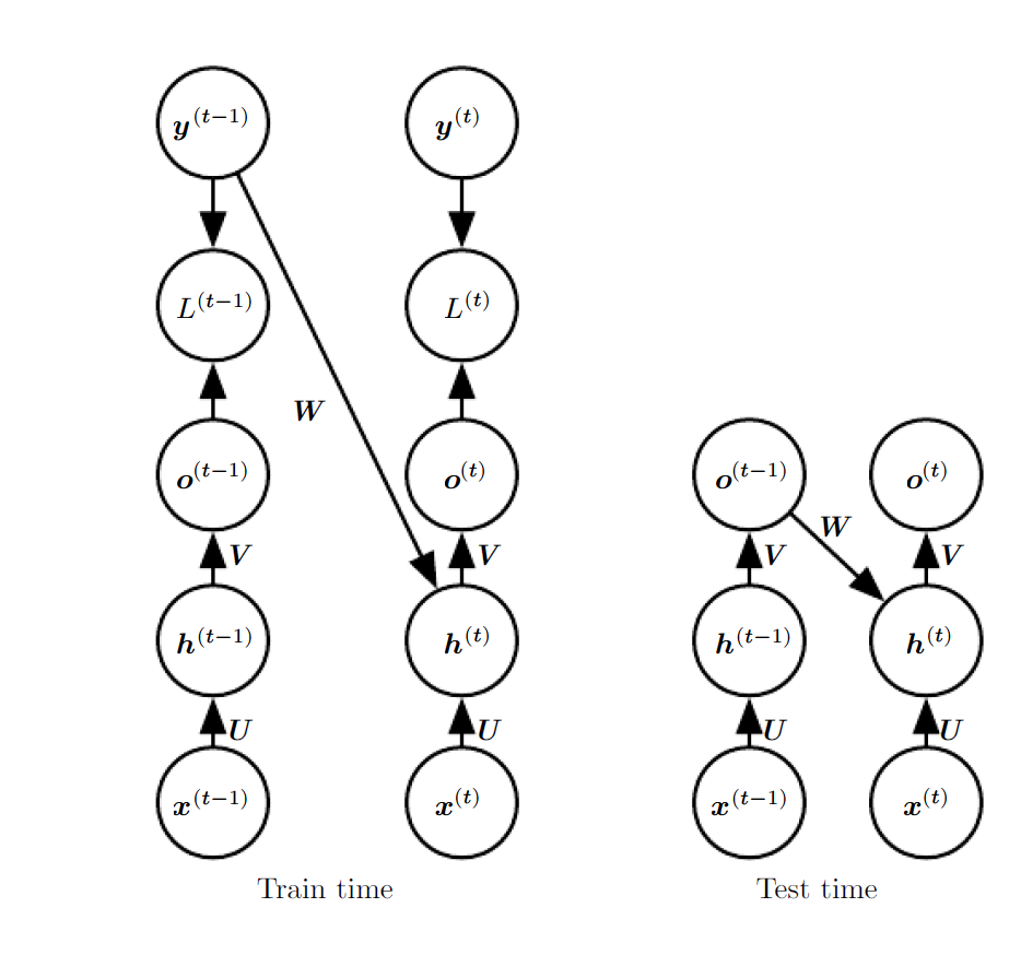
Teacher Forcing and Networks with Output Recurrence

RNNs are expensive to train. The runtime is \(O(\tau)\) and cannot be reduced by parallelization because the forward propagation graph is inherently sequential (i.e calculation of \(\mathbf{h}^t\) depends on \(\mathbf{h}^{t-1}\), the total loss is sum of per-timestep loss and per-timestep loss has to calculate in order); each time step may only be computed after the previous one. States computed in the forward pass must be stored until they are reused during the backward pass, so the memory cost is also \(O(\tau)\).

To reduce computational and memory cost, one way is to remove the hidden to hidden recurrence by a target to hidden recurrence. Thus, for any loss function based on comparing the prediction at time \(t\) to the training target at time \(t\), all time steps are decoupled and can be parallelized (because the loss calculation at each time step \(t\) is no longer dependent on \(\mathbf{h}^{t-1}\), it only depends on \(\mathbf{y}^{t-1}\)).

This technique is called teacher forcing. Teacher forcing is a procedure that emerges from the maximum likelihood criterion, in which during training the model receives the ground truth output \(\mathbf{y}^{t-1}\) as input at time \(t\). It can be applied to train models that have connections from the output at one time step to the value computed in the next time step.

The disadvantage of strict teacher forcing arises if the network is going to be later used in an open-loop model, with the network outputs fed back as input. In this case, there is a gap between training and testing. One approach to collapse this gap is to mitigate the gap between the inputs seen at train time and the inputs seen at test time randomly chooses to use generated values or actual data values as input.

Backward Pass

The backward propagation for RNN is called back propagation through time:

Assume we have RNN structure as forward pass (gradients are reshaped to column vectors, \(\nabla_{\mathbf{v}} L = (\frac{\partial L}{\partial \mathbf{v}})^T\)). Then, for any time step \(t\) \[\frac{\partial L}{\partial L^t} = 1\]

\[\frac{\partial L}{\partial L^t} \frac{\partial L^t}{\partial \mathbf{\hat{y}}^t} \frac{\partial \mathbf{\hat{y}}^t}{o^t_i} = \hat{y}^t_i - y^t_i\]

Then the gradient for hidden units in last time step \(\tau\) is:

\[(\frac{\partial L}{\partial \mathbf{o}^t} \frac{\partial \mathbf{o}^t}{\partial \mathbf{h}^t})^T = V^T \frac{\partial L}{\partial \mathbf{o}^t}\]

Work our way backwards for \(t = 1, ...., \tau - 1\), since \(\mathbf{h}^t\) is descendants of both \(\mathbf{o}^t\) and \(\mathbf{h}^{t+1}\). We have:

\[(\frac{\partial L}{\partial \mathbf{h}^t})^T = (\frac{\partial L}{\partial \mathbf{o}^t}\frac{\partial \mathbf{o}^t}{\partial \mathbf{h}^t})^T + (\frac{\partial L}{\partial \mathbf{h}^{t+1}}\frac{\partial \mathbf{h}^{t+1}}{\partial \mathbf{h}^t})^T\]

Since \(\frac{\partial \tanh (\mathbf{a}^{t+1})}{\partial \mathbf{a}^{t+1}}\) is a diagonal matrix with \(1 - \tanh (h^{t+1}_i)^2\) terms in the diagonal, we can denoted it as:

\[\begin{aligned} \frac{\partial \tanh (\mathbf{a}^{t+1})}{\partial \mathbf{a}^{t+1}} &= diag (1 - \tanh (\mathbf{h}^{t+1})^2)\\ \end{aligned}\]

\[\implies (\frac{\partial \mathbf{h}^{t+1}}{\partial \mathbf{h}^{t+1}})^T = W^T diag (1 - \tanh (\mathbf{h}^{t+1})^2)\]

Then:

\[(\frac{\partial L}{\partial \mathbf{h}^t})^T = V^T (\frac{\partial L}{\partial \mathbf{o}^t})^T + W^T diag (1 - \tanh (\mathbf{h}^{t+1})^2)(\frac{\partial L}{\partial \mathbf{h}^{t+1}})^T\]

Recall that in RNN, all parameters are shared, so \(\frac{\partial L}{\partial W}\) represents the contribution of \(W\) to the value of \(L\) due to all edges in the computational graph. To resolve the ambiguity, we index \(W\) by time \(W^t\) where \(W^t\) is copy of \(W\) and only used in time step \(t\). Thus, we can use \(\frac{\partial f}{\partial W^t}\) to denote the contribution of the weights to the gradient at time step t:

\[(\frac{\partial L}{\partial \mathbf{c}})^T = \sum^{\tau}_{t=1} I (\frac{\partial L}{\partial \mathbf{o}^t})^T = \sum^{\tau}_{t=1} (\frac{\partial L}{\partial \mathbf{o}^t})^T\] \[(\frac{\partial L}{\partial \mathbf{b}})^T = \sum^{\tau}_{t=1} diag (1 - \tanh (\mathbf{h}^{t})^2) I (\frac{\partial L}{\partial \mathbf{h}^{t}})^T = \sum^{\tau}_{t=1} diag (1 - \tanh (\mathbf{h}^{t})^2) (\frac{\partial L}{\partial \mathbf{h}^{t}})^T \] \[\frac{\partial L}{\partial V}= \sum^{\tau}_{t=1} (\frac{\partial L}{\partial \mathbf{o}^t})^T (\mathbf{h}^t)^T\] \[\frac{\partial L}{\partial W}= \sum^{\tau}_{t=1} diag (1 - \tanh (\mathbf{h}^{t})^2) (\frac{\partial L}{\partial \mathbf{h}^{t}})^T (\mathbf{h}^{t-1})^T\] \[\frac{\partial L}{\partial U}= \sum^{\tau}_{t=1} diag (1 - \tanh (\mathbf{h}^{t})^2) (\frac{\partial L}{\partial \mathbf{h}^{t}})^T (\mathbf{x}^{t})^T\]

Bidirectional RNNs

The RNN structures so far only captures information from the past (i.e output at time step \(t\) is calculated using \((\mathbf{x}^1, \mathbf{y}^1) , ...., (\mathbf{x}^{t-1}, \mathbf{y}^{t-1}), \mathbf{x}^t\)). It is sometimes useful to have another RNN that moves from the back of the sequence.

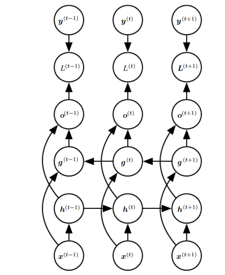
• \(\mathbf{h}^t\) is the hidden units of sub-RNN that moves forward through time.
• \(\mathbf{g}^t\) is the hidden units of sub-RNN that moves backward through time.
• \(\mathbf{o}^t\) is calculated using both \(\mathbf{h}^t\), \(\mathbf{g}^t\) but is more sensitive to input values around \(t\) without having to specify a fixed-size window around \(t\).

Encoder-Decoder

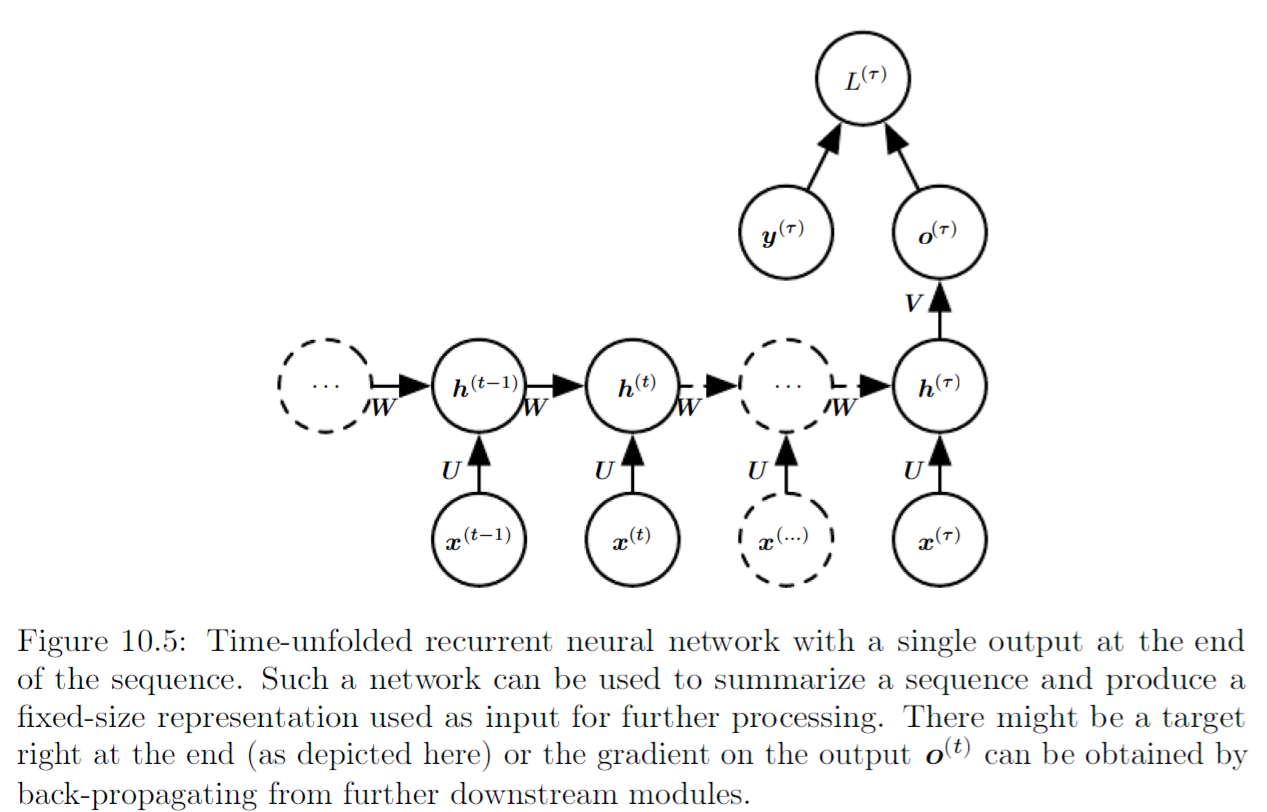
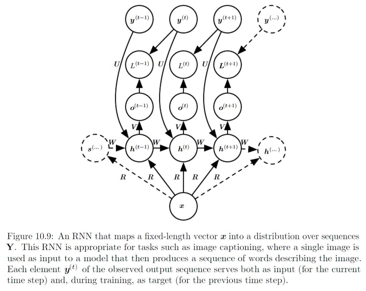
We know that we can use RNN to encode inputs to a fixed length vector, and we know that we can map a fixed-size vector to a sequence. Previously, we have one output corresponding to one input, the input sequence and the output sequence have same length. Using encoder-decoder or sequence to sequence structure, we can train an encoder RNN to process the input sequence \(\mathbf{x} = (\mathbf{x}^1, ...., \mathbf{x}^{n_x})\) and emits a context vector \(C\), then this context vector \(C\) is mapped to an output sequence \(\mathbf{y} = (\mathbf{y}^1, ....., \mathbf{y}^{n_y})\) which is not necessarily of the same length using a decoder RNN.

In the sequence to sequence structure, the two RNNs are trained jointly to maximize the average of log conditional probability \(\log P_{\mathbf{Y}}(\mathbf{y}^{1} ,...., \mathbf{y}^{n_y} | \; \mathbf{x}^1 , ...., \mathbf{x}^{n_x})\) or minimize the cross entropy over all sequence in the training set. The last state \(\mathbf{h}_{n_x}\) of the encoder RNN is typically used as a representation \(C\) of the input sequence that is provided as input to the decoder RNN.

One clear limitation of this architecture is when the context \(C\) output by the encoder RNN has a dimension that is too small to properly summarize a long sequence. Thus, rather than a fixed length of context vector, a variable-length sequence should be used which is the result of attention that learns to associate elements of the sequence \(C\) to elements of the output sequence.

Gated RNN

Gated RNN includes long short-term memory and networks based on the gated recurrent unit. Gated RNNs are based on the idea of creating paths through time that have derivatives that neither banish nor explode. Gated RNNs did this with connection weights that may change at each time step.

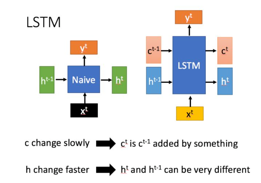
LSTM

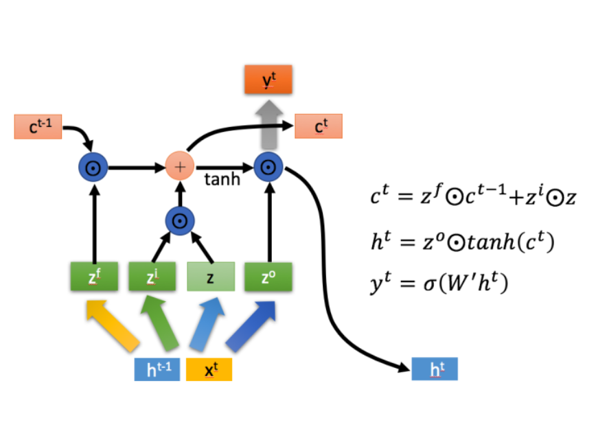
Instead of a unit that simply applies an element wise linearity to the affine transformation of inputs and recurrent units, LSTM recurrent networks have LSTM cells that have an internal recurrence in addition to the outer recurrence of the RNN. Each cell has more parameters and a system of gating units that controls the flow of information. The most important component is the state unit \(\mathbf{c}^{(t)}_i\) that is a linear function.

For each timestep \(t\):

\[\mathbf{z} = \tanh (W * [\mathbf{x}^t, \mathbf{h}^{t-1}] + \mathbf{b})\]

\[\mathbf{z}^i = \sigma(W^i * [\mathbf{x}^t, \mathbf{h}^{t-1}] + \mathbf{b}_i)\]

\[\mathbf{z}^f = \sigma(W^f * [\mathbf{x}^t, \mathbf{h}^{t-1}] + \mathbf{b}_f)\]

\[\mathbf{z}^o = \sigma(W^o * [\mathbf{x}^t, \mathbf{h}^{t-1}] + \mathbf{b}_o)\]

Where \((W^i, \mathbf{b}_i), (W^f, \mathbf{b}_f), (W^o, \mathbf{b}_o)\) are the parameters associated with input gate, forget gate, output gate respectively. Notice each gate is a value between \([0, 1]\). The internal states is computed as:

\[\mathbf{c}^{t} = \mathbf{z}^f \odot \mathbf{c}^{t-1} + \mathbf{z}^i \odot \mathbf{z}\]

We can see that if \(\mathbf{z}^f = 1\) and \(\mathbf{z}^i = 1\), we transfer the current and past information directly to next layer without any transformation.

Then:

\[\mathbf{h}^t = \mathbf{z}^o \odot \tanh (\mathbf{c}^t)\]

\[\mathbf{y}^t = \sigma (V\mathbf{h}^t + \mathbf{b}_y)\]

In LSTMs, you have the state \(\mathbf{c}^t\). The derivative there is of the form:

\[\frac{\partial \mathbf{c}^{t^{\prime}}}{\partial \mathbf{c}^{t}} = \prod^{t^{\prime} - t}_{k=1} \sigma (\mathbf{v}_{t+k})\]

Where \(\mathbf{v}_{t+k}\) is the input to the forget gate. We can see that compare with the \(\frac{\partial \mathbf{h}^{t^{\prime}}}{\partial \mathbf{h}^{t}}\) in RNN, we do not have \(W^T\) term. Thus, we have somewhat solved the vanishing gradient problem (at least one path the gradient is not vanishing). However, we still have vanishing gradient problem in LSTM, but not as much as RNN (no gradient of sigmoid or multiplication of \(W\)).

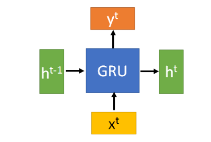
GRU

The main difference with the LSTM is that a single gating unit simultaneously controls the forgetting factor and the decision to update the state unit so we have less parameters.

The input and output to GRU is same as RNN

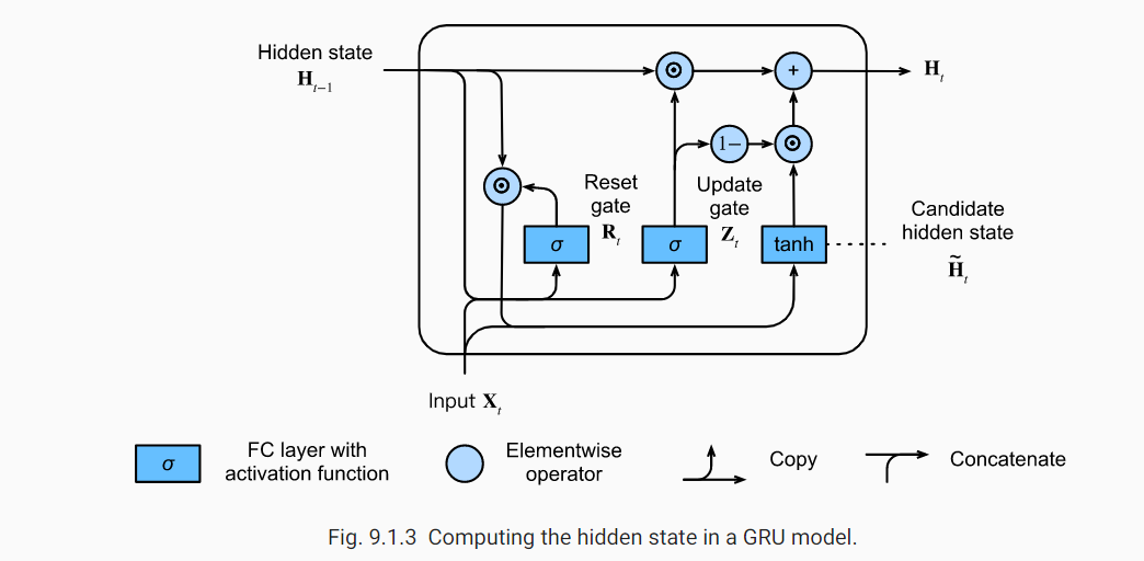
GRU has two gates at each timestep \(t\):

• Reset gate \(\mathbf{r}^{t}\): \[\mathbf{r}^{t} = \sigma(W^r * [\mathbf{x}^t, \mathbf{h}^{t-1}] + \mathbf{b}_r)\]

• Update gate \(\mathbf{u}^t\): \[\mathbf{u}^t = \sigma(W^u * [\mathbf{x}^t, \mathbf{h}^{t-1}] + \mathbf{b}_u)\]

The hidden unit update equation is:

\[\mathbf{h}^{t-1, \prime} = h^{t-1} \odot \mathbf{r}\]

\[\mathbf{h}^{t, \prime} = \tanh(W * [\mathbf{h}^{t-1, \prime}, \mathbf{x}_t] + \mathbf{b})\]

\[\mathbf{h}^{t} = \mathbf{u}^t \odot \mathbf{h}^{t-1} + (1 - \mathbf{u}^t) \odot \mathbf{h}^{t, \prime}\]

Where \(\mathbf{h}^{t, \prime}\) is the candidate at timestep \(t\) that has some new information \(\mathbf{x}^t\) and old information \(\mathbf{h}^{t-1, \prime}\). When \(\mathbf{u}_t = 1\) we simply keep the old information and the new information \(\mathbf{x}_t\) is ignored. In contrast, whenever \(Z_t\) is close to 0, the candidate is used inplace.

In summary:

• Reset gates help capture short-term dependencies in sequences (by integrating part of past information with new information to produce the candidate).
• Update gates help capture long-term dependencies in sequences.

Ref

https://zhuanlan.zhihu.com/p/32085405

https://zhuanlan.zhihu.com/p/32481747

https://stats.stackexchange.com/questions/185639/how-does-lstm-prevent-the-vanishing-gradient-problem

https://d2l.ai/chapter_recurrent-modern/gru.html