LGBM
LightGBM: A Highly Efficient Gradient Boosting Decision Tree
Background
GBDT
GBDT is an ensemble model of decision trees, which are trained in sequence. In each iteration, GBDT learns the decision trees by fitting the negative gradients (also known as residual errors).
The main cost in GBDT lies:
- Learning the decision trees (finding the best split points) when there is large number of features and samples.
- Histogram based algorithm buckets continuous feature values into discrete bins and uses these bins to construct feature histograms during training. It finds the best split points based on the feature histogram, the criterion is calculated at the interval boundaries. It costs \(O(N \times M)\) for histogram building and \(O(\text{Number of bins} \times M)\) for split point finding. Since number of bins is much smaller than number of data points, histogram building will dominate the computational complexity.
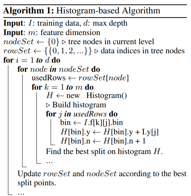
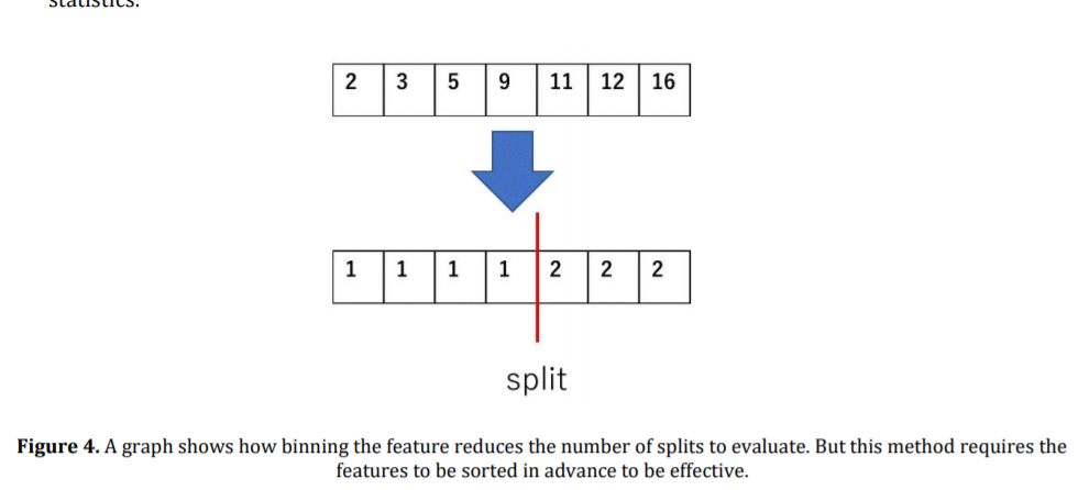
- Pre-sorted algorithm sorts the values of each numeric attribute, and evaluates the criterion at each possible split point to find the splitting point with the minimum criterion. The sorting requires \(O(n\log (n))\).
- Histogram based algorithm buckets continuous feature values into discrete bins and uses these bins to construct feature histograms during training. It finds the best split points based on the feature histogram, the criterion is calculated at the interval boundaries. It costs \(O(N \times M)\) for histogram building and \(O(\text{Number of bins} \times M)\) for split point finding. Since number of bins is much smaller than number of data points, histogram building will dominate the computational complexity.
- Number of Samples:
- Down sampling the data instance (i.e weights, random subsets), most of the algorithms are based on adaboost which has weights but not GBDT which does not have weights natively. Random subsets hurt the performance.
- Number of Features:
- PCA to remove weak correlated features (depends on assumption that features contain significant redundancy which might not always be true in practice)
Gradient-based One-Side Sampling
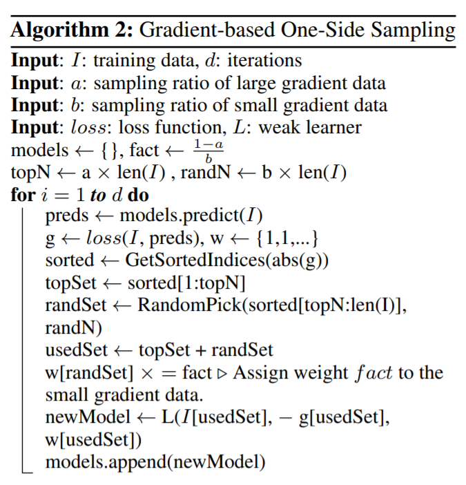
In AdaBoost, the sample weight serves as a good indicator for the importance of data instances. In GBDT, gradient for each data instance provides us with useful information for data sampling. That is, if an instance is associated with a small gradient, the training error for this instance is small and it is already well-trained. A straightforward idea is to discard those data instances with small gradients. However, the data distribution will be changed by doing so. To avoid this problem, GOSS keeps all the instances with large gradients and performs random sampling on the instances with samll gradients.
In order to compensate the influence to the data distribution, when computing the information gain, GOSS introduces a constant multiplier for the data instances with samll gradients. Specifically, GOSS:
- Firstly sorts the data instances according to the absolute value of their gradients.
- Selects the top \(a \times 100%\) instances.
- Then it randomly samples \(b \times 100%\) from the rest of the data.
- Amplifies the sampled data with small gradients by a constant \(\frac{1 - a}{b}\) when calculating the criterion to normalize the sum of the gradients.
Exclusive Feature Bundling
High-dimensional data are usually very sparse. The sparsity of the feature space provides us a possibility of designing a nearly lossless approach to reduce the number of features. Specifically, in a sparse feature space, many features are mutually exclusive (they never take nonzero values simultaneously), we can safely bundle these features into a single feature. In this way, the complexity of histogram building changes from \(O(N \times M)\) to \(O(N \times \text{Number of bundles})\). Then we can significantly speed up the training of GBDT without hurting the accuracy.
Which Features to Bundle
Partitioning features into smallest number of exclusive bundles is NP-hard, thus it is impossible to find an exact solution within polynomial time. Thus, a greedy algorithm which can produce reasonable good results are being used. Furthermore, we can allow a small fraction of conflicts which is controlled by \(\gamma\) (there are usually quite a few features, although not 100% mutually exclusive, also rarely take nonzero values simultaneously) to have an even smaller number of feature bundles and further improve the computational efficiency. For small \(\gamma\), we will be able to achieve a good balance between accuracy and efficiency.
Intuitively, it:
- Builds a graph with features as vertices and weighted edges as total conflicts between features (Edge only occurs when two features are not mutually exclusive).
- Sort the features by their degrees (Number of edges)
- Check each feature in the ordered list and either append it to existing list (if total conflicts between feature and bundle less than \(\gamma\)) or create a new bundle.
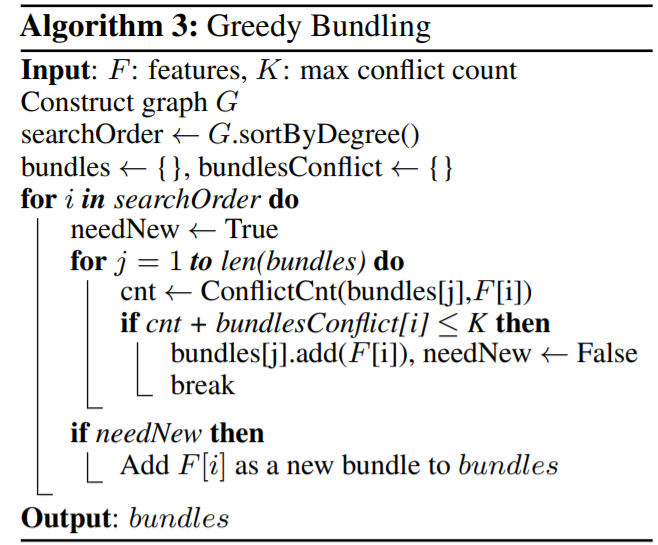
The time complexity of algorithm 3 is \(O(M^2)\) and it is only processed once before training. This complexity is acceptable when the number of features is not very large.
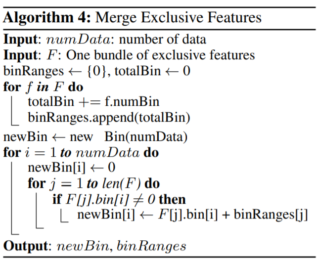
How to Construct the Bundle
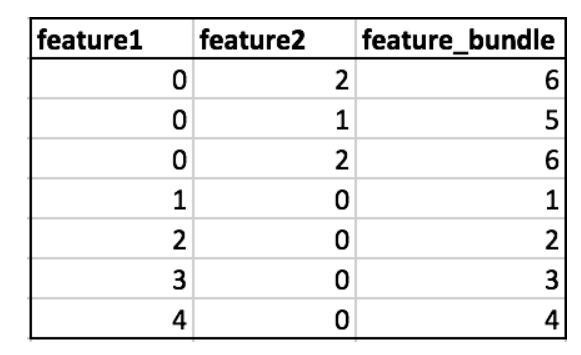
The key is to ensure that the values of the original features can be identified from the feature bundles. This can be done by adding offsets to the original values of the features:
- Calculate the offset to be added to every feature in feature bundle.
- Iterate over every data instance and feature.
- Initialize the new bucket as zero for instances where all features are zero.
- Calculate the new bucket for every non zero instance of a feature by adding respective offset to original bucket of that feature
Ref
https://www.researchgate.net/publication/351133481_Comparison_of_Gradient_Boosting_Decision_Tree_Algorithms_for_CPU_Performance
https://papers.nips.cc/paper/2017/file/6449f44a102fde848669bdd9eb6b76fa-Paper.pdf
https://robotenique.github.io/posts/gbm-histogram/
https://www.aaai.org/Papers/KDD/1998/KDD98-001.pdf