Sequential Data

In some cases, we have i.i.d assumptions to allow use to express the likelihood function as the product over all data points of the probability distribution evaluated at each data point. However, in some cases namely sequential data, we may not have i.i.d samples.

Markov Models

To express the sequential dependence of the samples, we can relax the i.i.d assumption and one of the simplest ways to do this is to consider a Markov Model. First of all, without loss of generality, we can use the product rule to express the joint distribution for a sequence of observations in the form:

\[P(X_1, ...., X_n) = \prod^N_{n=1} P(X_n | X_1, ..., X_{n-1})\]

If we assume that each of the conditional distributions on the right-hand side is independent of all previous observations except the most recent, we obtain the first-order Markov Chain, which can depicted as graphical model:

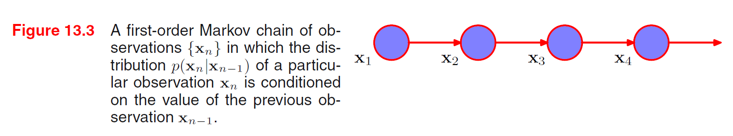
The joint distribution for a sequence of \(N\) observations under this model is given by:

\[P(X_1, ..., X_N) = P(X_1) \prod^{N}_{n=2} P(X_n | X_{n-1})\]

Thus, if we use such a model to predict the next observation in a sequence, the distribution of predictions will depend only on the value of the immediately preceding observation and will be independent of all earlier observations. In most applications of such models, the conditional distributions \(P(X_n | X_{n-1})\) that define the model will be constrained to be equal, corresponding to a assumption of a stationary time series. The model is then known as the homogeneous Markov Chain (All conditional distribution share the same parameters).

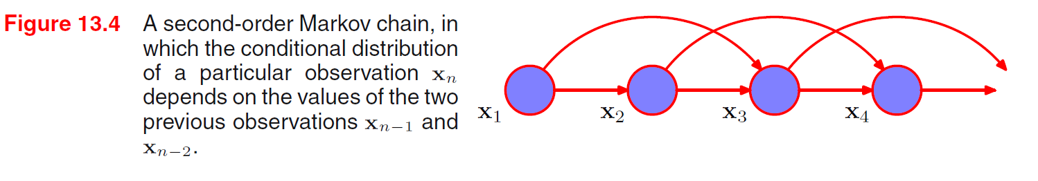
However, first-order Markov model is still restrictive. For many sequential observations, we anticipate that the trends in the data over several successive observations will provide important information in predicting the next value. One way to allow earlier observations to have an influence is to move to higher-order Markov chains, the second-order Markov chain is given by:

\[P(X_1, ..., X_N) = P(X_1) P(X_2 | X_1) \prod^{N}_{n=3} P(X_n | X_{n-1}, X_{n-2})\]

Suppose we wish to build a model for sequences that is not limited by the Markov assumption to any order and yet that can be specified using a limited number of free parameters. We can achieve this by introducing additional latent variables to permit a rich class of models to be constructed out of simple components, as we did with mixture distributions.

For each observation \(\mathbf{X}_n\), we introduce a corresponding latent random vector \(\mathbf{Z}_n\) which may be of different type or dimensionality to the observed variable. We now assume that it is the latent variables that form a Markov chain, giving rise to the graphical structure known as state space model. It satisfies the key conditional independence properties that \(\mathbf{Z}_{n-1}, \mathbf{Z}_{n+1}\) are independent given \(\mathbf{Z}_n\) so that:

\[\mathbf{Z}_{n+1} \perp \!\!\! \perp \mathbf{Z}_{n-1} \;|\; \mathbf{Z}_n\]

The joint distribution of the model is:

\[P(\mathbf{X}_1, ...., \mathbf{X}_{N}, \mathbf{Z}_1, ...., \mathbf{Z}_{N}) = P(\mathbf{Z}_1) \prod^N_{n=1} P(\mathbf{X}_n | \mathbf{Z}_n) \prod^{N}_{n=2} P(\mathbf{Z}_n | \mathbf{Z}_{n-1})\]

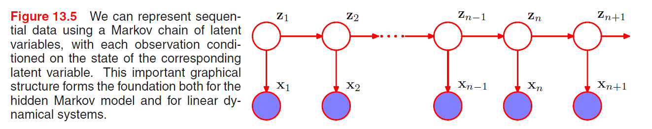
Using the d-separation criterion, we see that there is always a path connecting any two observed variables \(\mathbf{X}_n\) and \(\mathbf{X}_{n+1}\) via the latent variable, so the predictive distribution \(P(\mathbf{X}_{n+1} | \mathbf{X}_{1} , ..., \mathbf{X}_{n})\) does not have any conditional dependence properties so it depends on all previous variables.

There are two important models for sequential data:

1. Hidden Markov Model: If the latent variables are discrete.
2. Linear Dynamical System: If the latent variables, observed variables are Gaussian with a linear-Gaussian dependence of the conditional distributions on their parents.

Hidden Markov Models

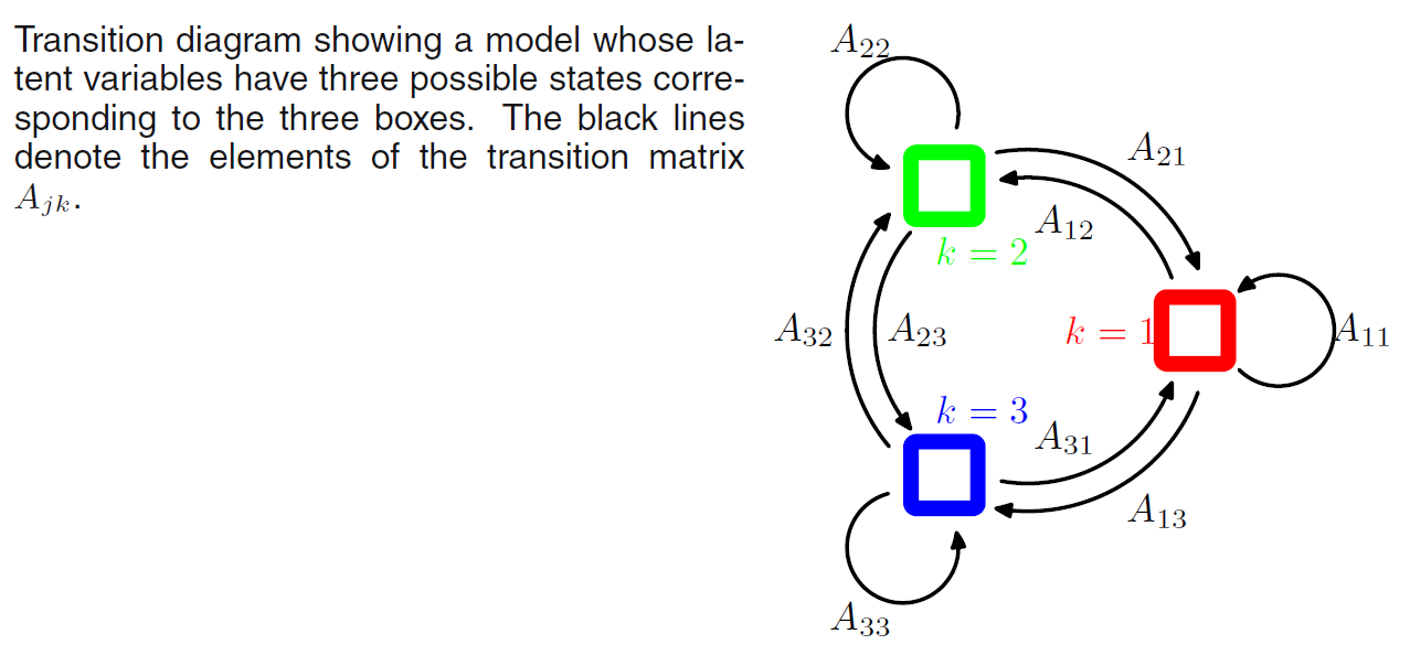
The hidden markov model can be viewed as specific instance of the state space model with discrete latent variables. It can also be viewed as an extension of a mixture model in which the choice of mixture component for each observation is not selected independently but depends on the choice of component for the previous observation.

It is convenient to use 1-of-\(K\) coding scheme for the latent variables \(\mathbf{Z}_n\). We now allow the probability distribution of \(\mathbf{Z}_n\) to depend on the state of previous latent variable \(\mathbf{Z}_{n-1}\) through a conditional probability distribution \(P(\mathbf{Z}_{n} | \mathbf{Z}_{n-1})\). Since, we want to express the dependency of each element of \(\mathbf{Z}_n\) on each element of \(\mathbf{Z}_{n-1}\), we introduce a \(K \times K\) matrix of probabilities that we denote by \(\mathbf{A}\), the element of which are known as transition probabilities:

\[A_{jk} = P(Z_{nk} = 1 | Z_{n-1, j}) = 1\]

And because they are probabilities:

\[\sum^K_{k=1} A_{jk} = 1\]

\[0 \geq A_{jk} \leq 1\]

We can write the conditional distribution explicitly in the form:

\[P(\mathbf{Z}_{n} | \mathbf{Z}_{n-1}, \mathbf{A}) = \prod^K_{k=1}\prod^{K}_{j=1} A_{jk}^{Z_{nk}Z_{n-1, \;j}}\]

The initial latent node \(\mathbf{Z}_1\) is special in that it does not have a parent node, and so it has a marginal distribution \(P(\mathbf{Z}_1)\) represented by a vector of probabilities that represents the initial probabilities \(\boldsymbol{\pi}\):

\[\pi_k = P(Z_{1k} = 1)\] \[\sum^{K}_{k=1} \pi_k = 1\] \[P(\mathbf{Z}_1 | \boldsymbol{\pi}) = \prod^K_{k=1} \pi_k^{Z_{1k}}\]

Lastly, the specification of the probabilistic model is completed by defining the conditional distribution of observed variables \(P(\mathbf{X}_n | \mathbf{Z}_n, \boldsymbol{\phi})\), where \(\boldsymbol{\phi} = \{\boldsymbol{\phi}_1, ...., \boldsymbol{\phi}_K\}\) is a set of parameters governing the distribution. These distributions are called emissino distribution and might be given by Gaussian if the elements of \(\mathbf{X}\) are continues random variables or by conditioanl probability tables if \(\mathbf{X}\) are discrete. Since the distribution depends on the values of \(\mathbf{Z}\) which has \(K\) possible states, We can define the emission distribution as:

\[P(\mathbf{X}_n | \mathbf{Z}_n, \boldsymbol{\phi}) = \prod^K_{k=1} P(\mathbf{X}_n | \boldsymbol{\phi}_k)^{Z_{nk}}\]

In this case, we focus on Homogeneous models for which all the conditional distributions governing the latent variables share the same parameters \(\mathbf{A}\) and similarly all of the emission distributions share the same parameters \(\boldsymbol{\phi}\), so the joint distribution is:

\[P(\mathbf{X}_1, ...., \mathbf{X}_{N}, \mathbf{Z}_1, ...., \mathbf{Z}_{N} | \boldsymbol{\theta}) = P(\mathbf{D}, \mathbf{H} | \boldsymbol{\theta}) = P(\mathbf{Z}_1 | \boldsymbol{\pi}) \prod^N_{n=1} P(\mathbf{X}_n | \mathbf{Z}_n, \boldsymbol{\phi}) \prod^{N}_{n=2} P(\mathbf{Z}_n | \mathbf{Z}_{n-1}, \mathbf{A})\]

Where \(\boldsymbol{\theta} = \{\boldsymbol{\pi}, \boldsymbol{\phi}, \boldsymbol{A}\}\)

Maximum Likelihood for HMM

If we have observed a dataset \[\mathbf{D} = \{\mathbf{x}_1, ...., \mathbf{x}_N\}\], we can determine the parameters of an HMM using maximum likelihood method. The likelihood function is obtained from the joint distribution by marginalizing over the latent variables:

\[L(\boldsymbol{\theta} ;\; \mathbf{D}) = \sum_{\mathbf{H}} P(\mathbf{D}, \mathbf{H} | \; \boldsymbol{\theta}) = P(\mathbf{D} | \; \boldsymbol{\theta}) = \prod^N_{n=1} P(\mathbf{x}_n |\; \boldsymbol{\theta})\]

This is similar to the mixture distribution with latent variable in EM, we have a summation inside the log for log likelihood which is much difficult to work with, direct maximization of the log likelihood function will therefore lead to complex expressions with no closed-form solutions. Thus, one way to solve the problem is to use EM algorithm to find an efficient framework for maximizing the likelihood function in HMM.

The EM algorithm starts with some initial selection for the model parameters, which we denote by \(\boldsymbol{\theta}^{old}\):

1. E step:
   • We take these parameter values and find the posterior distribution of the latent variables: \[P(\mathbf{H} | \mathbf{X}, \boldsymbol{\theta}^{old})\]
   • We then evaluate the expectation of complete log likelihood function over the posterior distribution of the latent variables as a function of new parameters \(\boldsymbol{\theta}\): \[Q(\boldsymbol{\theta}, \boldsymbol{\theta}^{old}) = E_{\mathbf{H} | \mathbf{D}, \boldsymbol{\theta}^{old}}[\ln P(\mathbf{D}, \mathbf{H} | \boldsymbol{\theta}) | \mathbf{D}, \boldsymbol{\theta}^{old}]\]
   • We can rewrite the log likelihood as: \[\begin{aligned} Q(\boldsymbol{\theta}, \boldsymbol{\theta}^{old}) &= \sum_{\mathbf{H}} P(\mathbf{H} | \mathbf{D}, \boldsymbol{\theta}^{old}) \ln P(\mathbf{D}, \mathbf{H} | \boldsymbol{\theta})\\ &= \sum^{K}_{k=1}P(Z_{1k} = 1 | \mathbf{D}, \boldsymbol{\theta}^{old}) \ln P(Z_{1k} = 1| \boldsymbol{\pi}) + \sum^N_{n=2}\sum^{K}_{j=1}\sum^{K}_{k=1} P(Z_{nk}, Z_{n-1, j} | \mathbf{D}, \boldsymbol{\theta}^{old}) \ln P(Z_{nk} | Z_{n-1, j}) + \sum^{N}_{n=1}\sum^{K}_{k=1} P(Z_{nk} = 1 | \mathbf{D}, \boldsymbol{\theta}^{old}) \ln P(\mathbf{X}_n| \boldsymbol{\phi}_k, Z_{nk}=1)\\ &= \sum^{K}_{k=1} \gamma(Z_{nk})\ln \pi_k + \sum^N_{n=2}\sum^{K}_{j=1}\sum^{K}_{k=1} \xi(Z_{nk}, Z_{n-1, j})\ln A_{jk} + \sum^{N}_{n=1}\sum^{K}_{k=1} \gamma(Z_{nk}) \ln P(\mathbf{X}_n| \boldsymbol{\phi}_k, Z_{nk}=1) \end{aligned}\] Where \(\gamma (Z_{nk}) = P(Z_{1k} = 1 | \mathbf{D}, \boldsymbol{\theta}^{old})\) and \(\xi(Z_{nk}, Z_{n-1, j}) = P(Z_{nk}, Z_{n-1, j} | \mathbf{D}, \boldsymbol{\theta}^{old}) \ln P(Z_{nk} | Z_{n-1, j})\)
   • Our goal is to evaluate these posterior probabilities \(\gamma, \xi\) efficiently
2. M step:
   • We maximize \(Q(\boldsymbol{\theta}, \boldsymbol{\theta}^{old})\) w.r.t the parameters \(\boldsymbol{\theta}\) in which we treat posterior probabilities as constant:

Ref

PRML Chapter 13