Time Series (1)

Time Series (Introduction)

Characteristics of Time Series

The primary objective of time series analysis is to develop mathematical models that provide plausible descriptions for sample data with time correlations. In order to provide a statistical setting for describing the character of data that seemingly fluctuate in a random fashion over time, we assume a time series can be defined as a collection of random variables indexed according to the order they are obtained in time. In general, a collection of random variables \(\{X_t\}\) indexed by \(t\) is referred to as a stochastic process. In this text, \(t\) will typically be discrete and vary over the integers.

Example of Series:

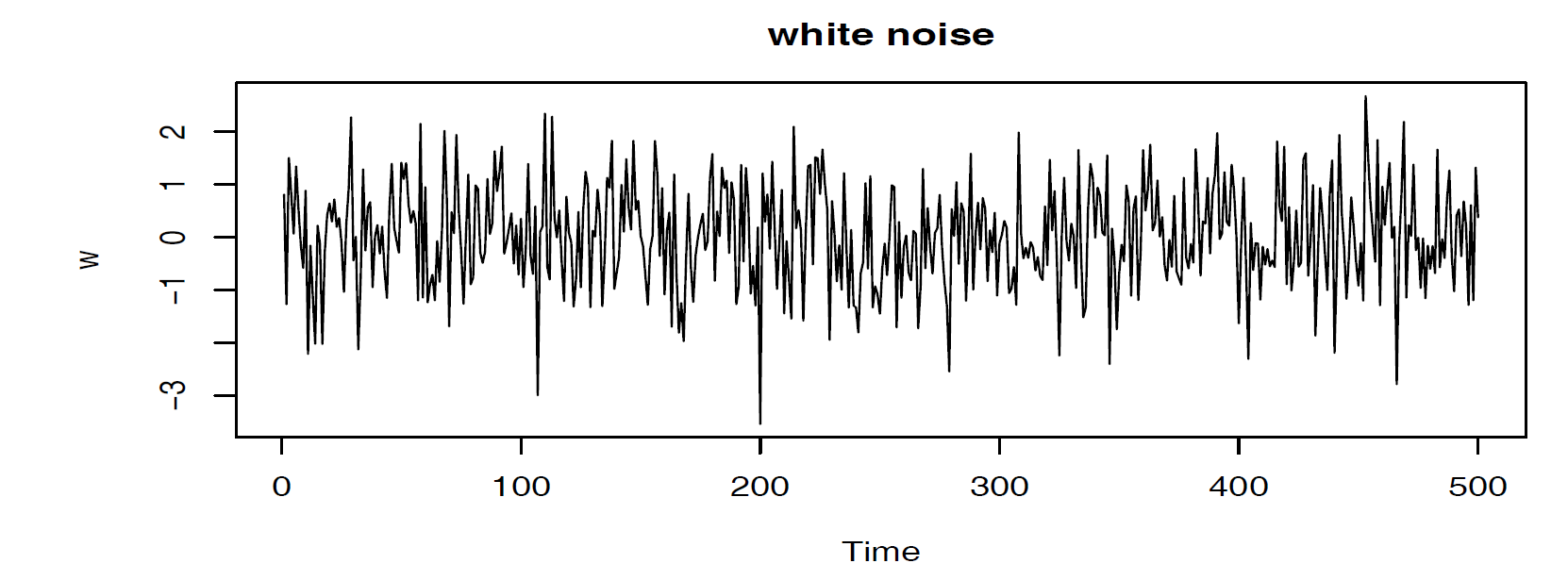
White Noise: A collection of uncorrelated, independent and identically distributed random variables \(W_t\) with mean 0 and finite variance \(\sigma^2_w\). A particular useful white noise is Gaussian white noise, that is \(W_t \overset{i.i.d}{\sim} N(0, \sigma^2_w)\)

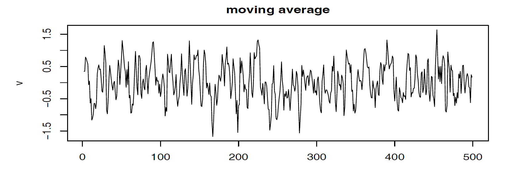
Moving Average: We might replace the white noise series \(W_t\) by a moving average that smooths the series: \[V_t = \frac{1}{3} (W_{t-1} + W_{t} + W_{t+1})\] This introduces a smoother version of white noise series, reflecting the fact that the slower oscillations are more apparent and some of the faster oscillations are taken out.

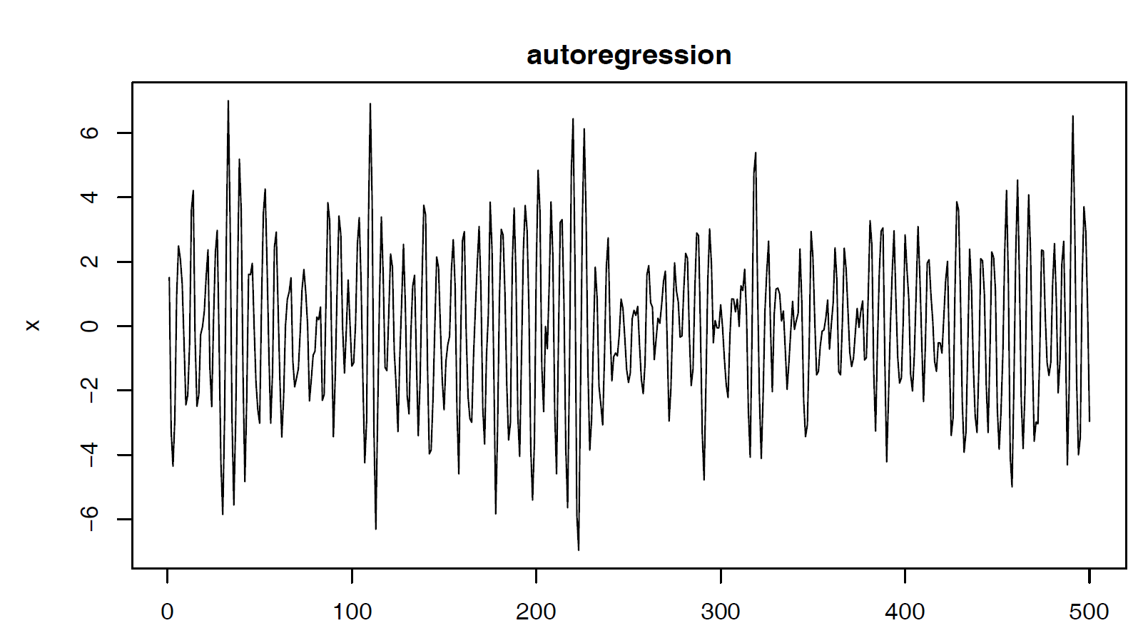
Autoregressions: Suppose we consider the white noise series \(W_t\) as input and calculate the output using the second-order equation: \[X_t = X_{t-1} - 0.9 X_{t-2} + W_t\] For \(t=1, ..., 500\). We can see the periodic behavior of the series.

Autocorrelation and Cross-Correlation

A complete description of a time series with \(N\) random variables at arbitrary integer time points \(t_1, ..., t_N\) is given by joint distribution function (joint CDF), evaluated as the probability that the values of the series are jointly less than the \(N\) constants \(c_1, ..., c_N\):

\[F_{X_{t_1}, ..., X_{t_N}}(c_1, ...., c_N) = P(X_{t_1} \leq c_1, ..., X_{t_N} \leq c_N)\]

In practice, the multidimensional distribution function cannot usually be written easily unless the random variables are jointly normal. It is an unwieldy tool for displaying and analyzing time series data. On the other hand, the marginal distribution functions:

\[F_{X_t} (x_t) = P(X_t \leq x_t)\]

or the corresponding marginal density functions:

\[f_{X_t} (x_t) = \frac{\partial F_{X_t} (x_t)}{\partial x_t}\]

And The Mean Function:

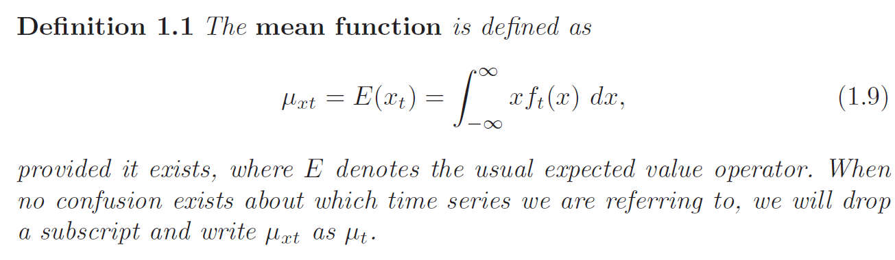
When they exist, are often informative for examining the marginal behavior of the series.

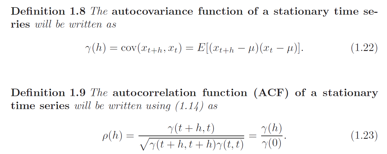
Autocovariance

The autocovariance measures the linear dependence between two points on the same series observed at different times:

1. Very Smooth series exhibit autocovariance functions that stay large even when \(t\) and \(s\) are far apart
2. Very Choppy series tend to have auto covariance functions that are nearly zero for large separations.

Autocorrelation

The ACF measures the linear predictability of the series at time \(t\), say \(X_t\), using only the value \(X_s\). iF we can predict \(X_t\) perfectly from \(X_s\) through a linear relationship \(X_t = \beta_0 + \beta_1 X_s\), then the correlation will be \(+1\) or \(-1\) depends on the sign of \(\beta_1\). Hence, we have a rough measure of the ability to forecast the series at time \(t\) from the value at time \(s\).

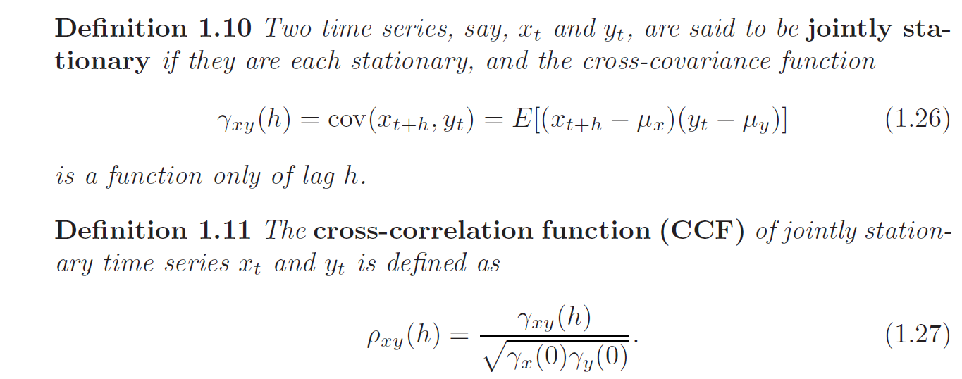
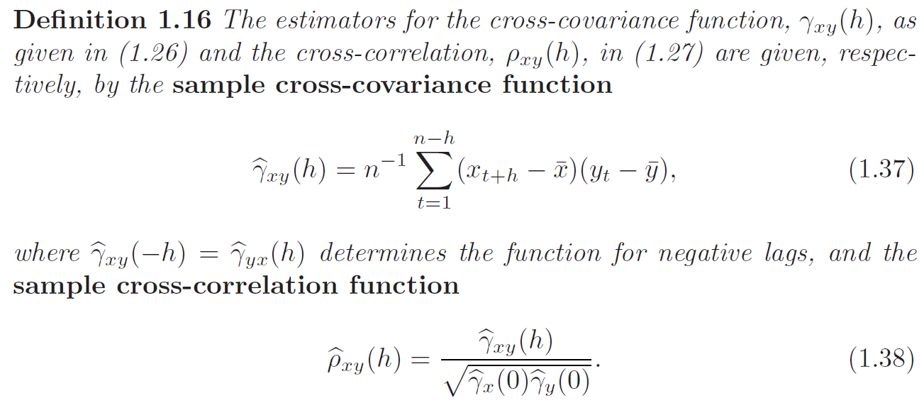
Cross-covariance and Cross-correlation

Often, we want to measure the predictability of another series (different components) \(Y_t\) from the series \(X_s\). Assuming both series have finite variances, we have the following definition:

We can easily extend the idea to multivariate time series where each sample contains r attributes:

\[X_{t} = <X_{t1}, ...., X_{tR}>\]

The extension of autocovariance is then:

\[\gamma_{jk} (s, t) = E[(X_{sj} - \mu_{sj}) (X_{tk} - \mu_{tk})]\]

Stationary Time Series

There may exist a sort of regularity over time in the behavior of a time series.

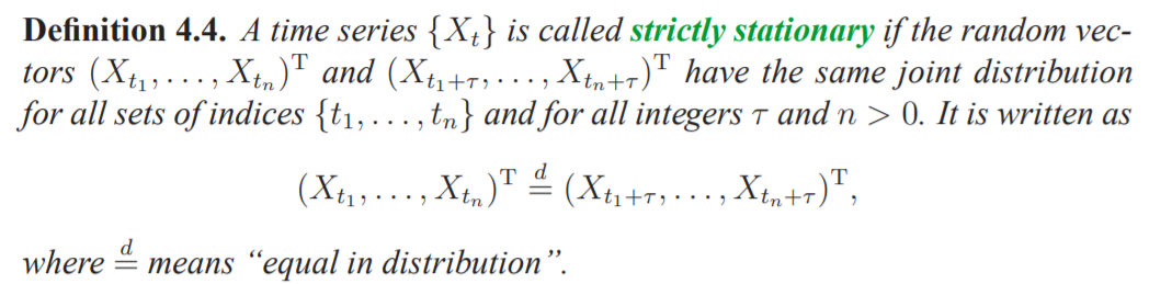
Strictly Stationarity

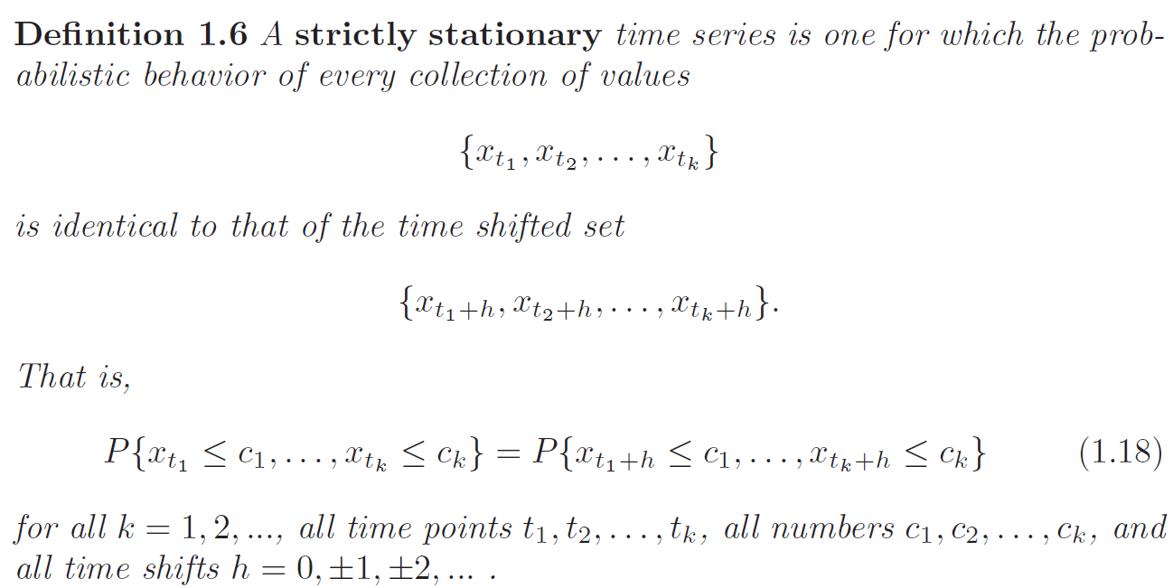
When \(k = 1\), we can conclude that random variables are identically distributed and mean is constant regardless of time:

\[P(X_s \leq c) = P(X_t \leq c) = P(X_1 \leq c), \;\; \forall c, s, t \implies E[X_s] = E[X_t] = \mu\]

When \(k = 2\), we can conclude that for any pairs of \(s, t\), the joint distribution is identical regardless of time:

\[P(X_{s} \leq c_1, X_{t} \leq c_2) = P(X_{s + h} \leq c_1, X_{t} \leq c_2), \; \forall h, c_1, c_2\]

\((X_1, X_2), (X_3, X_4), (X_8, X_9)\) are identically distributed

\((X_2, X_4), (X_3, X_5), (X_8, X_{10})\) are identically distributed

Thus, if the variance function of the process exists, we have autocovariance function of the series \(\{X_t\}\) satisfies:

\[\gamma(s, t) = \gamma(s + h, t + h)\]

Same conclusions for all possible values of \(k\). The version of strictly stationarity is too strong for most applications and it is difficult to assess strict stationarity from a single data set.

Weak Stationarity

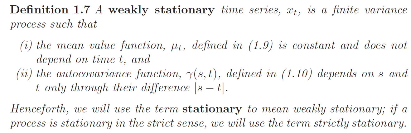
Thus, \(\forall s, t, h\):

1. \(E[X_t] = E[X_s] = \mu\)
2. \(\gamma(s, s + h) = Cov(X_s, X_{s+h}) = Cov(X_0, X_{h}) = \gamma(0, h) \;\) or \(\; \gamma(s, t) = \gamma(s + h, t + h)\)

From above, we can clearly see that a strictly stationary, finite variance, time series is also stationary. The converse is not true unless there are further conditions.

Several Properties:

1. \(|\gamma(h)| \leq Var[X_t] = \gamma(0)\)
2. \(\gamma(h) = \gamma(-h)\)
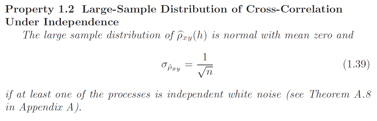
3. \(\rho_{xy}(h) = \rho_{yx}(-h)\)
4. \(\gamma(\cdot)\) is non-negative definite, for all positive integers \(N\) and vector \(<X_1, ..., X_N>^T \in \mathbb{R}^N\): \[\sum^N_{i=1} \sum^N_{j=1} X_i \gamma(i - j) X_j \geq 0\]

Gaussian Process

If a Gaussian Process is weakly stationary then it is also strictly stationary.

Linear Process

A Linear process \(X_t\) is a stationary process defined to be a linear combination of white noise variates \(X_t\) and is given by:

\[X_t = \mu + \sum^\infty_{j=-\infty} \psi_j W_{t-j}, \quad \sum^{\infty}_{j=-\infty} |\psi_j| < \infty\]

The autocovariance function for linear process is:

\[\gamma(h) = \sigma^2_w \sum^\infty_{j=-\infty} \psi_{j+h} \psi_j\]

Estimation of Correlation

If a time series is stationary, the mean function is constant, so that we can estimate it by the sample mean:

\[\bar{X} = \frac{1}{N} \sum^N_{t=1} X_t\]

The sum runs over a restricted range because \(X_{t+h}\) is not available for \(t+h > n\). Thus, this estimator is a biased estimator of \(\gamma(h)\). The normalizing term \(\frac{1}{N}\) guarantees a non-negative definite function because autocovariance function is non-negative definite for stationary series, so it is preferred over \(\frac{1}{N - h}\).

The sample autocorrelation function has a sampling distribution that allows us to assess whether the data comes from a completely random or white series or whether correlations are statistically significant at some lags.

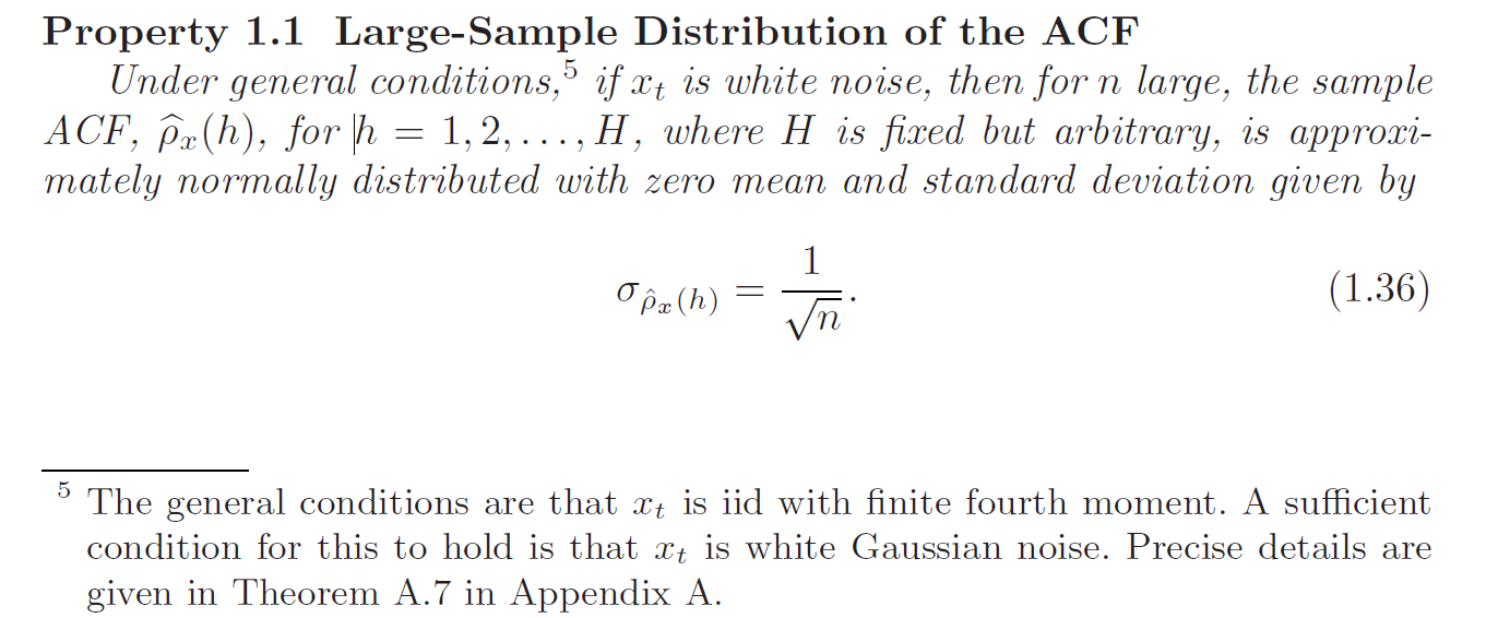
Based on the property, we obtain a rough method of assessing whether peaks in \(\hat{\rho}(h)\) are significant by determining whether the observed peak is outside the interval \(0 \pm \frac{2}{\sqrt{N}}\) (95% of data should be within 2 s.e of a standard normal distribution).

Vector-Valued and Multidimensional Series

Consider the notion of a vector time series \(\mathbf{X}_t = <X_{t1}, ...., X_{tp}>^T \in \mathbb{R}^p\) that contains \(p\) univariate time series. For the stationary case, the mean vector \(\boldsymbol{\mu}\) is:

\[\boldsymbol{\mu} = E[\mathbf{X}_t] = <\mu_{t1}, ...., \mu_{tp}>^T\]

And the \(p\times p\) autocovariance matrix is denoted as:

\[\Gamma (h) = E[(\mathbf{X}_{t+h} - \boldsymbol{\mu}) (\mathbf{X}_t - \boldsymbol{\mu})^T]\] \[\gamma_{ij} (h) = E[(X_{t+h, i} - \mu_i) (X_{t, j} - \mu_j)], \;\; i,j = 1, ...., p\]

Since, \(\gamma_{ij}(h) = \gamma_{ji} (-h)\):

\[\Gamma(-h) = \Gamma^T(h)\]

The sample autocovariance matrix is defined as:

\[\hat{\Gamma}(h) = \frac{1}{N}\sum^{N-h}_{t=1} (\mathbf{X}_{t+h} - \bar{\mathbf{X}}) (\mathbf{X}_t - \bar{\mathbf{X}})^T\] \[\hat{\Gamma} (-h) = \hat{\Gamma}^T(h)\]

Where \(\bar{\mathbf{X}} = \frac{1}{N} \sum^{N}_{t=1} \mathbf{X}_t\) is the sample mean vector.

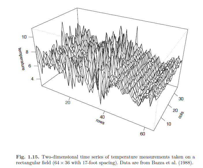
In many applied problems, an observed series may be indexed by more than one time alone. For example, the position in space of an experimental unit might be described by two coordinates. We may proceed in these cases by defining a multidimensional process (does not have multiple dependent variables as multivariate case)\(\mathbf{X}_\mathbf{s}\) as a function of the \(r \times 1\) vector \(\mathbf{s} = <s_1, ..., s_r>^T\), where \(s_i\) denotes the coordinate of the \(i\)th index. The autocovariance function of a stationary multidimensional process, \(X_{\mathbf{s}}\) can be defined as a function of the multidimensional lag vector, \(\mathbf{h} = <h_1, ..., h_r>^T\) as:

\[\gamma (\mathbf{h}) = E[(X_{\mathbf{s} + \mathbf{h}}) - \mu) (X_{\mathbf{s}} - \mu)]\]

Where \(\mu = E[X_{\mathbf{s}}]\)

The multidimensional sample autocovariance function is defined as:

\[\hat{\gamma}(\mathbf{h}) = (S_1S_2...S_r)^{-1} \sum_{s_1} .... \sum_{s_r} (X_{\mathbf{s} + \mathbf{h}} - \bar{X})(X_{\mathbf{s}} - \bar{X})\]

Where each summation has range \(1 \leq s_i \leq S_i - h_i, \;\; \forall i=1, ..., r\)

\[\bar{X} = (S_1 ... S_r)^{-1} \sum_{s_1} ... \sum_{s_r} X_{\mathbf{s}}\]

Where each summation has range \(1 \leq s_i \leq S_i, \;\; \forall i=1, ..., r\)

The multidimensional sample autocorrelation function follows:

\[\hat{\rho}(\mathbf{h}) = \frac{\hat{\gamma}(\mathbf{h})}{\hat{\gamma}(\mathbf{0})}\]

EDA

In general, it is necessary for time series data to be stationary, so averaging lagged products over time will be a sensible thing to do (fixed mean). Hence, to achieve any meaningful statistical analysis of time series data, it will be crucial that the mean and the autocovariance functions satisfy the conditions of stationarity.

Trend

Detrend

The easiest form of nonstationarity to work with is the trend stationary model wherein the process has stationary behavior around a trend. We define this as:

\[X_t = \mu_t + Y_t\]

Where \(X_t\) are the observations, \(\mu_t\) denotes the trend, and \(Y_t\) is a stationary process. Strong trend will obscure the behavior of the stationary process \(Y_t\). Hence, there is some advantage to removing the trend as a first step in an exploratory analysis of such time series. The steps involved are to obtain a reasonable estimate of the trend component, and then work with the residuals:

\[\hat{Y}_t = X_t - \hat{\mu}_t\]

\(\hat{\mu} = -11.2 + 0.006t \implies \hat{Y}_t = X_t + 11.2 - 0.006t\)

Differencing

Differencing can be used to produce a stationary time series. The first difference operator is a linear operator denoted as:

\[\nabla X_t = X_t - X_{t-1}\]

If \(\mu_t = \beta_1 + \beta_2 t\), then:

\[\nabla X_t = (\mu_t + Y_t) - (\mu_{t-1} + Y_{t-1}) = \beta_2 + Y_t - Y_{t-1} \implies Z_t = X_t - \beta_2\]

Where \(Z_t = Y_t - Y_{t-1}\) is a stationary time series given \(Y_t\) is a stationary time series.

One advantage of differencing over detrending to remove trend is that no parameters are estimated in the differencing operation. One disadvantage, however, is that differencing does not yield an estimate of the stationary process \(Y_t\) as detrending. If an estimate of \(Y_t\) is essential, then detrending may be more appropriate. If the goal is to coerce the data to be stationarity, then differencing is more appropriate.

Backshift Operator

Backshift Operator is linear. We can rewrite first difference as:

\[\nabla X_t = X_t - X_{t-1} = (1 - B) X_t\]

And second difference as:

\[\nabla^2 (X_t) = \nabla (\nabla X_t) = (1 - B)^2 X_t\]

Transformations

If a time series presents nonstationary as well as nonlinear behavior, transformations may be useful to equalize the variability over the length of a single series. A particular useful transformation is the log transformation:

\(Y_t = \log X_t\)$

Which tends to suppress larger fluctuations that occur over portions of the series where the underlying values are larger.

Smoothing

Smoothing is useful in discovering certain traits in a time series, such as long-term trend and seasonal components.

Moving Average Smoother

If \(X_t\) represents the observations, then

\[M_t = \sum^k_{j=-k} a_j x_{t-j}\]

Where \(a_j = a_{j} \geq 0\) and \(\sum^k_{j=-k} a_j = 1\) is a symmetric moving average of the data centered at \(X_t\).

Kernel Smoothing

Kernel smoothing is a moving average smoother that uses a weight function or kernel to average the observations:

\[\hat{f}_t = \sum^N_{i=1} w_i(t) X_i\]

\[w_i (t) = \frac{K(\frac{t - i}{b})}{\sum^N_{j=1} K(\frac{t - j}{b})}\]

Where \(b\) is a bandwidth parameter, the wider the bandwidth, the smoother the result. \(K(\cdot)\) is a kernel function that is often the normal kernel:

\[K(z) = \frac{1}{\sqrt{2\pi}}\exp(\frac{-z^2}{2})\]

Lowess and Nearest Neighbor Regression

Another approach to smooth a time series is nearest neighbor regression. The technique is based on \(k\)-nearest neighbors linear regression, wherein one uses the neighbouring data \(\{X_{t-\frac{k}{2}}, ..., X_t, ..., X_{t + \frac{k}{2}}\}\) to predict \(X_t\) using a linear regression. The result is \(\hat{f}_t\).

Lowess is a method of smoothing that is complex but similar to nearest neighbor regression:

1. A certain proportion of nearest neighbors to \(X_t\) are included in a weighting scheme, values closer to \(X_t\) in time get more weight.
2. A robust weighted regression is used to predict \(X_t\) and obtain the smoothed estimate of \(f_t\).

Visualization

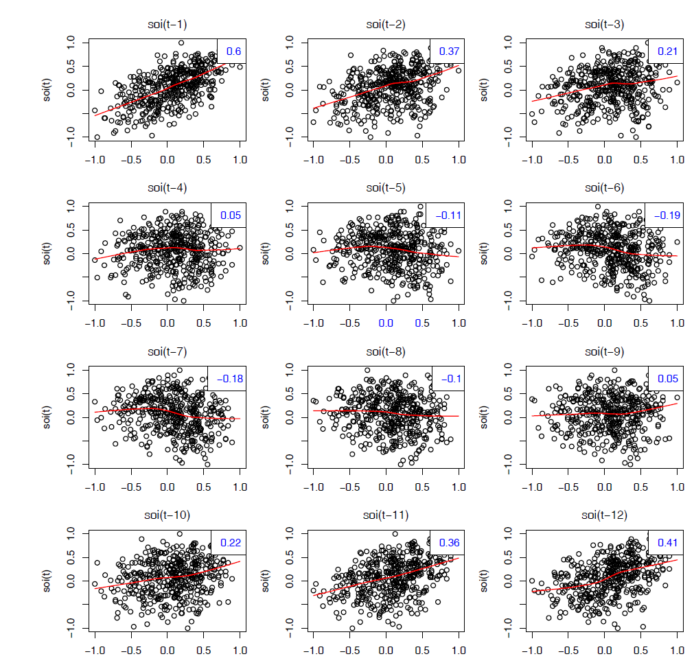
Lagged Scatterplot Matrices (Non-linearity and Lag correlation)

In the definition of the ACF, we are essentially interested in relations between \(X_t\) and \(X_{t-h}\). The autocorrelation function tells us whether a substantial linear relation exists between the series and its own lagged values. The ACF gives a profile of the linear correlation at all possible lags and shows which values of \(h\) leads to the best predictability. The restriction of this idea to linear predictability, however, may mask a possible nonlinear relation between current values and past values. Thus, to check for nonlinear relationship of this form, it is convenient to display a lagged scatterplot matrix.

The plot displays values \(S_t\) on the vertical axis plotted against \(S_{t-h}\) on the horizontal axis.The sample autocorrelations are displayed in the upper right-hand corner and superimposed on the sctterplots are locally weighted scatterplot smoothing lines (LOWESS) that can be used to help discover any nonlinearities.

Ref

Time Series Analysis and Its Applications With R Examples by Robert H.Shumway and David S.Stoffer

https://www.math-stat.unibe.ch/e237483/e237655/e243381/e281679/files281692/Chap13_ger.pdf