Time Series (2)
Time Series (ARIMA)
Autoregressive Moving Average Models (ARMA)
Autoregressive Models
Autoregressive models are based on the idea that the current value of the series \(X_t\) can be explained as a function of \(p\) past values, \(X_{t-1}, X_{t-2}, ..., X_{t-p}\) where \(p\) determines the number of steps into the past needed to forecast the current value.
An autoregressive model of order \(p\), abbreviated \(AR(p)\) with \(E[X_t] = 0\), is of the form:
\[X_t = \phi_1 X_{t-1} + \phi_2 X_{t-2} + ... + \phi_p X_{t-p} + W_t\]
Where \(X_t\) is stationary, \(\phi_1, ..., \phi_p \neq 0\) are constants, \(W_t\) is a Gaussian white noise series with mean zero and variance \(\sigma^2_w\). We assume above equation \(X_t\) has mean zero, if it has non zero mean \(\mu\), we can replace it by:
\[X_t - \mu = \phi(X_{t-1} - \mu) + \phi_2(X_{t-2} - \mu) + ... + \phi_p (X_{t-p} - \mu) + W_t\] \[\implies X_t = \alpha + \phi_1 X_{t-1} + \phi_2 X_{t-2} + ... + \phi_p X_{t-p} + W_t\]
Where \(\alpha = \mu(1 - \phi_1 - ... - \phi_p)\).
We can also use the backshift operator to rewrite the zero mean \(AR(p)\) process as:
\[(1 - \phi_1 B - \phi_2 B^2 - ... - \phi_p B^p) X_t = W_t\]
or using autoregressive operator:
\[\phi(B)X_t = W_t\]
Autoregressive Operator
The Autoregressive operator is defined to be:
\[\phi_p(B) = 1 - \phi_1 B - \phi_2 B^2 - ... - \phi_p B^p\]
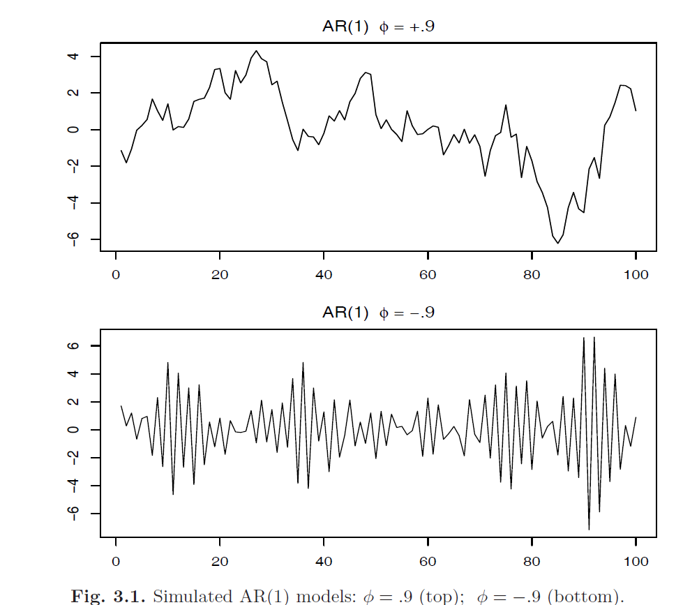
We can write the \(AR\) models as a linear process. Start with \(AR(1)\) with zero mean, given by \(X_t = \phi_1 X_{t-1} + W_t\) and iterating backwards \(k\) times, we get:
\[\begin{aligned} X_t &= \phi_1 X_{t-1} + W_t = \phi (\phi X_{t-2} + W_{t-1}) + W_t\\ &= \phi^2 X_{t-2} + \phi W_{t-1} + W_t\\ & \; .\\ & \; .\\ & \; .\\ &= \phi^k X_{t-k} + \sum^{k-1}_{j=0}\phi^j W_{t-j}\\ \end{aligned}\]If we keep iterating, we have:
\[X_t = \sum^{\infty}_{j=0} \phi^j W_{t-j}\]
If \(|\phi_j| < 1\), we have the infinite sum defined and the process is a linear process (with \(\psi_j = \phi^j\)).
To calculate the mean, autocovariance and autocorrelation of the \(AR(1)\) process:
Mean:
\[E[\sum^{\infty}_{j=0} \phi^j W_{t-j}] = 0\]
Autocovariacne
\[\gamma(h) = \sigma^2_w \sum^\infty_{j=0} \phi^{j + h} \phi^{j} = \sigma^2_w \phi^h \sum^\infty_{j=0} \phi^{2j} = \frac{\sigma^2_w \phi^h}{1 - \phi^2}, \;\; h \geq 0\]
Autocorrelation:
\[\rho(h) = \frac{\gamma(h)}{\gamma(0)} = \phi^h\]
Moving Average Models
The moving average model of order \(q\), abbreviated as \(MA(q)\), assumes the white noise \(W_t\) on the right-hand side of the defining equation are combined linearly to form the observed data.
The Moving Average or \(MA(q)\) model is defined to be:
\[X_t = W_t + \theta_1W_{t-1} + \theta_2 W_{t-2} + ... + \theta_q W_{t-q}\]
Where there are \(q\) lags in the moving average and \(\theta_1, ..., \theta_q (\theta_q \neq 0)\) are parameters. Assume \(W_{t}\) is a Gaussian white noise series with mean zero and variance \(\sigma^2_w\).
The system is the same as the linear process with \(\psi_j = \theta_j, \psi_0 = 1, \; \; \forall j=0, 1, ..., q\) and \(\psi_j = 0\) for all other values of \(j\).
Moving Average Operator
The Moving Average Operator is:
\[\theta_q(B) = 1 + \theta_1 B + \theta_2 B^2 + .... + \theta_q B^q\]
The model can be written in terms of operator:
\[X_t = \theta_q(B) W_t\]
Unlike the autoregressive process, the moving average process is stationary for any values of \(\theta\).
Consider the \(MA(1)\) model \(X_t = W_t + \theta W_{t-1}\). Then \(E[X_t] = 0\) and the autocovariance:
\[\gamma(0) = (\psi_0^2 + \psi_1^2)\sigma^2_w = (1 + \theta^2)\sigma^2_w\] \[\gamma(1) = (\psi_0\psi_1 + 0 * \psi_1) \sigma^2_w = \theta\sigma^2_w\] \[\gamma(i) = 0, \;\; \forall i > 1\]
The autocorrelation:
\[\rho(1) = \frac{\theta}{1 + \theta^2}\] \[\rho(i) = 0, \;\; \forall i > 1\]
In contrast with \(AR(1)\) model, the autocorrelation only exists between \(X_t, X_{t-1}\) and \(|\rho(1)| \leq 0.5, \; \forall \theta\)

Altogether: ARMA
We now proceed with the general development of autoregressive, moving average and mixed autoregressive moving average models for stationary series.
A time series \(\{X_t; \; t=0, \pm 1, \pm 2, ....\}\) is \(\mathbf{ARMA(p, q)}\) if it is stationary and:
\[X_t = \phi_1 X_{t-1} + ... + \phi_p X_{t-p} + W_t + \theta_1 W_{t-1} + .... + \theta_q W_{t-q}\] \[\phi(B)X_t = \theta(B) W_t\]
With \(W_t\) being a Gaussian white noise with mean zero, variance \(\sigma^2_w\) and \(\theta_q \neq 0\), \(\phi_q \neq 0\) and \(\sigma^2_w > 0\). The parameters \(p, q\) are called the autoregressive and moving average orders respectively. If \(X_t\) has non-zero mean \(\mu\), we set \(\alpha = \mu(1 - \phi_1 - .... - \phi_p)\) and write the model as:
\[X_t = \alpha + \phi_1 X_{t-1} + ... + \phi_p X_{t-p} + W_t + \theta_1 W_{t-1} + .... + \theta_q W_{t-q}\]
Problems with general definitions of \(\mathbf{ARMA(p, q)}\):
- Parameter redundant models
- Stationary AR models that depend on the future (Causal)
- MA models that are not unique (Invertibility)
To overcome these problems, we will require some additional restrictions on the model parameters.
AR and MA Polynomials
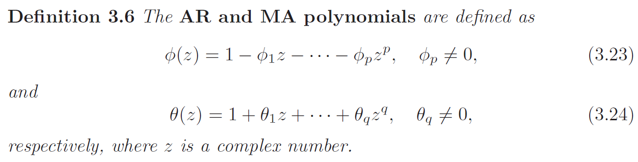
To address the parameter redundancy, we will henceforth refer to an \(ARMA(p, q)\) model to mean that it is in its simplest form. That is, in addition to the original definition, we will also require that \(\phi(z)\) and \(\theta(z)\) have no common factors (\(z\) is often \(B\) the backshift operator, we can treat \(B\) as complex number here).
The process \[X_t = 0.5X_{t-1} - 0.5W_{t-1} + W_t \implies (1 - 0.5B)X_t = (1 - 0.5B)W_t \implies X_t = W_t\] is not \(ARMA(1, 1)\) process because the original process has common factor \((1 - 0.5B)\). In its reduced form, \(X_t\) is a white noise.
Causality
An \(ARMA(p, q)\) model is said to be causal, if the time series \(\{X_t; t = 0, \pm 1, \pm 2 ...\}\) can be written as a one-sided linear process:
\[X_t = \sum^\infty_{j=0} \psi_jW_{t-j} = \psi (B) W_t\]
Where \(\psi(B) = \sum^\infty_{j=0} \psi_j B^j\) and \(\sum^\infty_{j=0} |\psi_j| < \infty\), we set \(\psi_0 = 1\)
Property 3.1 Causality of an \(ARMA(p, q)\) Process
An \(ARMA(p, q)\) model is causal if and only if \(\phi(z) \neq 0\) for \(|z| \leq 1\). The coefficient of the linear process above can be determined by solving:
\[\psi(z) = \sum^\infty_{j=0} \psi_j z^j = \frac{\theta(z)}{\phi(z)}, \;\; |z| \leq 1\]
Another way to phrase the property is that an \(ARMA(p, q)\) process is causal only when the roots of \(\phi(z)\) lie outside the unit circle:
\[\phi(z) = 0 \implies |z| > 1\]
Consider the \(AR(1)\) process: \[X_t = \phi X_{t-1} + W_t\] This process is causal only when \(|\phi| < 1\). Equivalently, the process is causal only when the root of \(\phi(z) = 1 - \phi z = 0\) is bigger than one in absolute value. That is: \[1 - \phi z = 0 \implies z = \frac{1}{\phi}\] Since \(|\phi| < 1\), we have \(|z| > 1\)
Invertible and Uniqueness
To address the problem of uniqueness, we choose the model that allows an infinite autoregressive representation.
An \(ARMA(p, q)\) model is said to be invertible, if the time series \(\{X_t; t = 0, \pm 1, \pm 2 ...\}\) can be written as:
\[\pi(B)X_t = \sum^\infty_{j=0} \pi_j X_{t-j} = W_t\]
Where \(\pi(B) = \sum^\infty_{j=0} \pi_j B^j\) and \(\sum^\infty_{j=0} |\pi_j| < \infty\). We set \(\pi_0 = 1\)
Property 3.2 Invertibility of an \(ARMA(p, q)\) Process
An \(ARMA(p, q)\) model is invertible if and only if \(\theta(z) \neq 0\) for \(|z| \leq 1\). The coefficient \(\pi_j\) above can be determined by solving:
\[\pi(z) = \sum^\infty_{j=0} \pi_j z^j = \frac{\phi(z)}{\theta(z)}, \;\; |z| \leq 1\]
Another way to phrase the property is that an \(ARMA(p, q)\) process is invertible only when the roots of \(\theta(z)\) lies outside the unit circle:
\[\theta(z) = 0 \implies |z| > 1\]
Consider the process: \[X_t = 0.4 X_{t-1} + 0.45 X_{t-2} + W_t + W_{t-1} + 0.25 W_{t-2}\] In operator form: \[\phi(B)X_t = \theta(B)W_t\] Where: \[\phi(B) = 1 - 0.4B - 0.45 B^2\] \[\theta(B) = 1 + B + 0.25 B^2\] At first, this appears to be an \(ARMA(2, 2)\) process: \[\phi(z) = (1 + 0.5z) (1 - 0.9z) \implies |z| > 1\] \[\theta(z) = (1 + 0.5z)^2 \implies |z| > 1\] however, the polynomial has common factor \((1 + 0.5z)\), so the model is not an \(ARMA(2, 2)\) process. After cancellation, the model is an \(ARMA(1, 1)\) model. It is causal and invertible. Using properties 3.2 and 3.1, we can find the coefficients for linear process: \[\phi(z) \psi(z) = \theta(z) \implies (1 - 0.9z) (\psi_0 + \psi z + ...) = (1 + 0.5z) \implies X_t = W_t + 1.4 \sum^\infty_{j=1} 0.9^{j-1}W_{t-j}\] \[\theta(z) \psi(z) = \phi(z) \implies X_t = 1.4\sum^\infty_{j=1} (-0.5)^{j-1} X_{t-j} + W_t\]
Difference Equations
The study of the behavior of \(ARMA\) process and their ACFs is greatly enhanced by a basic knowledge of difference equations.
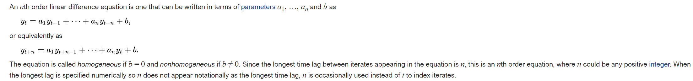
Homogeneous Difference Equation of Order 1
Suppose we have a sequence of numbers \(u_0, u_1, ....\) s.t:
\[u_n - \alpha u_{n-1} = 0, \;\; \alpha \neq 0, \; n = 1, 2, ....\]
This equation represents a homogeneous difference equation of order 1. To solve the equation, we write:
\[u_1 = \alpha u_0\] \[u_2 = \alpha u_1 = \alpha^2 u_0\] \[u_n = \alpha^n u_0\]
Given the initial condition \(u_0 = c\), we may solve \(u_n = \alpha^n c\). In operator notation:
\[u_n - \alpha u_{n-1} = 0 \implies (1 - \alpha B) u_n = 0\]
The polynomial associated with this is \(\alpha(z) = 1 - \alpha z\). We know that \((1 - \alpha z) = 0 \implies z = \frac{1}{\alpha} \implies \alpha = \frac{1}{z}\). Thus, a solution can be obtained given the initial condition \(u_0 = c\):
\[u_n = \alpha^n c = (z^{-1})^n c\]
If we know the root \(z\), we will know the solution to the equation. In other words, the solution ot the difference equation above depends only on the initial condition and the inverse of the root to the associated polynomial \(\alpha(z)\).
Homogeneous Difference Equation of Order 2
Suppose that the sequence satisfies:
\[u_n - \alpha_1 u_{n-1} - \alpha_2 u_{n-2} = 0, \;\; \alpha_2 \neq 0, \; n=2, 3, ...\]
This equation is a homogeneous difference equation of order 2. The corresponding polynomial is:
\[\alpha(z) = 1 - \alpha_1 z - \alpha_2 z^2\]
which has two roots say \(z_1, z_2\) s.t \(\alpha(z_1) = \alpha(z_2) = 0\). We will consider 2 cases:
Case 1: \(z_1 \neq z_2\)
In this case, the general solution to the difference equation is:
\[u_n = c_1 z_1^{-n} + c_2 z_2^{-n}\]
Given two initial conditions \(u_0, u_1\), we may solve for \(c_1, c_2\):
\[u_0 = c_1 + c_2\] \[u_1 = c_1 z_1^{-1} + c_2 z_2^{-1}\]
In case of distinct roots, the solution to the homogeneous difference equation of degree two is:
\[u_n = z_1^{-n} \times \text{(a polynomial in $n$ of degree $m_1 - 1$)} + z_2^{-n} \times \text{(a polynomial in $n$ of degree $m_2 - 1$)}\]
Where \(m_1\) is the multiplicity of the root \(z_1\) and \(m_2\) is the multiplicity of the root \(z_2\). In this case \(m_1 = m_2 = 1\) (zero degree polynomial is represented as \(c_1\) and \(c_2\))
Case 2: \(z_1 = z_2 = z_0\)
In this case, the general solution to the difference equation is:
\[u_n = z_0^{-n} (c_1 + c_2 n)\]
Given two initial conditions \(u_0, u_1\), we may solve for \(c_1, c_2\):
\[u_0 = c_1, u_1 = (c_1 + c_2)z_0^{-1}\]
In the case of repeated root, the solution is:
\[u_n = z_0^{-n} \times \text{(a polynomial in $n$ of degree $m_0 - 1$)}\]
Where \(m_0\) is the multiplicity of the root \(z_0\) that is \(m_0 = 2\) (first degree polynomial is represented as \(c_1 + c_2 n\))
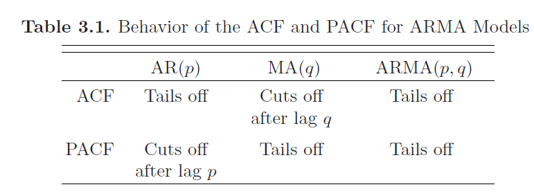
Autocorrelation and Partial Autocorrelation
For a causal \(ARMR(p, q)\) model, \(\phi(B)X_t = \theta(B)W_t\), where the roots of \(\phi(z)\) are outside of unit circle, write:
\[X_t = \sum^{\infty}_{j=0} \psi_j W_{t-j}\]
It follows immediately that \(E[X_t] = 0\) and the autocovariance function of \(X_t\) can be write as:
\[\gamma(h) = Cov(X_{t+h}, X_{t}) = \sigma^2_w \sum^{\infty}_{j=0} \psi_j \psi_{j+h}, \; \; h\geq 0\]
We could obtain a homogeneous difference equation direcrtly in terms of \(\gamma(h)\) to solve for the \(\psi\) weights. First, we write:
\[\begin{aligned} \gamma(h) &= Cov(X_{t+h}, X_{t}) \\ &= Cov(\sum^{p}_{j=1} \phi_j X_{t+h-j} + \sum^{q}_{j=0} \theta_j W_{t+h-j}, X_t)\\ &= \sum^{p}_{j=1} \phi_j Cov(X_{t+h-j}, X_t) + \sum^p_{j=0} \theta_j Cov(W_{t+h-j}, \sum^{\infty}_{k=0}\psi_k W_{t-k})\\ &= \sum^{p}_{j=1} \phi_j \gamma(h - j) + \sum^p_{j=h}\theta_j \sigma^2_w \psi_{j-h} \end{aligned}\]Where, white noise with different index has zero covariance:
\[Cov(W_{t+h-j}, \sum^{\infty}_{k=0}\psi_k W_{t-k}) = \psi_{j-h} \sigma^2_w\]
Then we can write the general difference equation of the autocovariance function:
\[\gamma(h) - \phi_1\gamma(h - 1) - ... - \phi_p\gamma(h - p) = 0, \;\; h \geq \max(p, q + 1)\]
With initial conditions:
\[\gamma(h) - \sum^{p}_{j=1} \phi_j \gamma(h - j) = \sum^p_{j=h}\theta_j \sigma^2_w \psi_{j-h}, \;\; 0 \leq h \leq \max(p, q)\]
Dividing the \(\gamma(h)\) by \(\gamma(0)\), we have the ACF.
Partial Autocorrelation Function (PACF)
Consider a causal \(AR(1)\) model \(X_t = \phi X_{t-1} + W_t\), the covariance function for lag 2 is:
\[\gamma(2) = \frac{\sigma^2_w \phi^2}{1 - \phi^2} = \sigma^2_w \gamma(0)\]
The correlation between \(X_t\) and \(X_{t-2}\) is not zero, as it would be for \(MA(1)\) process, because \(X_t\) is dependent on \(X_{t-2}\) through \(X_{t-1}\). Suppose we break this chain of dependence by removing the effect of \(X_{t-1}\), in other words, we consider the correlation between \(X_{t} - \phi X_{t-1}\) and \(X_{t-2} - \phi X_{t-1}\), because it is the correlation between \(X_t\) and \(X_{t-2}\) with the linear dependence of each on \(X_t\) removed. In this way, we have broken the dependence chain between \(X_t\) and \(X_{t-2}\):
\[Cov(X_{t} - \phi X_{t-1}, X_{t-2} - \phi X_{t-1}) = 0\]
Hence, the tool we need is partial autocorrelation, which is the correlation between \(X_s, X_t\) with everything in the middle removed.
The partial autocorrelation function (PACF) of a stationary process \(X_t\), denoted \(\phi_{hh}\), for \(h = 1, 2, ...\) is:
\[\phi_{11} = \rho(1)\] \[\phi_{hh} = Corr(X_{t+h} - \hat{X}_{t+h}, X_{t} - \hat{X}_{t}), \;\; h \geq 2\]
Where \(\hat{X}_{t+h}\) denotes the regression of a zero mean stationary time series \(X_{t+h}\) on \(\{X_{t+h-1}, ...., X_{t+1}\}\) which we write as:
\[\hat{X}_{t+h} = \beta_1 X_{t+h-1} + \beta_2 X_{t+h-2} + .. + \beta_{h-1} X_{t+1}\]
And \(\hat{X}_t\) denotes the regression of \(X_t\) on \(\{X_t, ...., X_{t+h-1}\}\):
\[\hat{X}_t = \beta_1 X_{t+1} + \beta_2 X_{t+2} + .. + \beta_{h-1} X_{t+h-1}\]
These \(\beta\) are the same for both regressions and are found by minimizing the expected mean squared error:
\[E[X_{t-h} - \sum^{h-1}_{j=1}\beta_j X_{t+j}]^2\]
Both \(X_{t+h} - \hat{X}_{t+h}\) and \(X_{t} - \hat{X}_{t}\) are uncorrelated with \(\{X_{t+1}, ..., X_{t+h-1}\}\). The PACF, \(\phi_{hh}\) is the correlation between \(X_{t+h}\) and \(X_t\) with the linear dependence of \(\{X_{t+1}, ..., X_{t+h-1}\}\) on each removed.
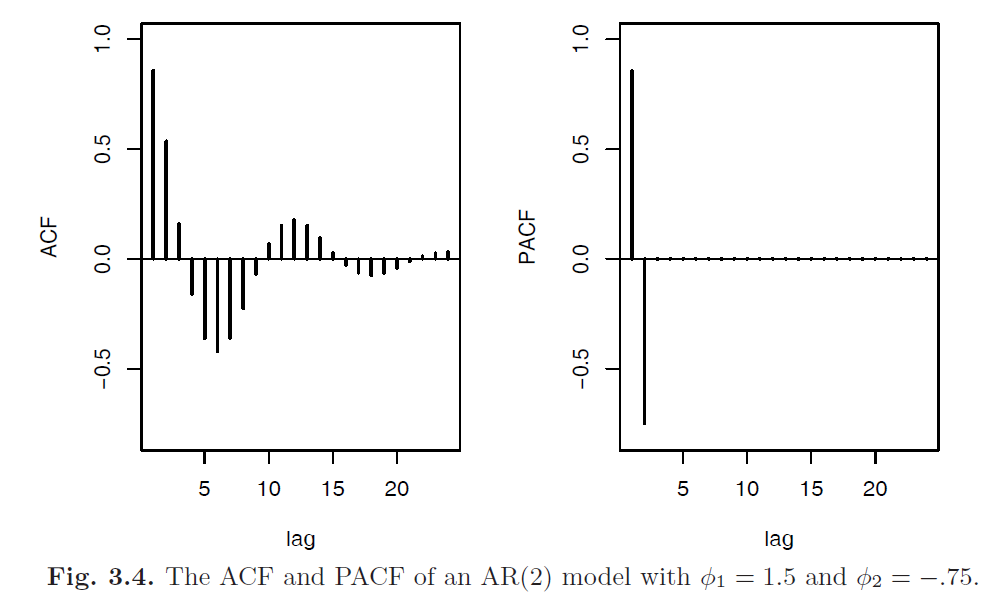
Consider the PACF of the \(AR(1)\) process given by \(X_t = \phi X_{t-1} + W_t\) with \(|\phi| < 1\). By definition, \(\phi_{11} = \rho(1) = \phi\). To calculate \(\phi_{22}\), consider regression of \(\hat{X}_{t+2} = \beta X_{t+1}\). We choose \(\beta\) to minimize: \[E[X_{t+2} - \hat{X}_{t+2}]^2 = E[(X_{t+2} - \beta X_{t+1})^2] - Var[X_{t+2} - \hat{X}_{t+2}] = \gamma(0) - 2 \beta \gamma(1) + \beta^2 \gamma(0)\] Taking the derivative w.r.t \(\beta\), setting the result to zero, we have: \[\beta = \frac{\gamma(1)}{\gamma(0)} = \rho(1) = \phi\] Hence, \[\phi_{22} = Corr(X_{t+2} - \hat{X}_{t+2}, X_t - \hat{X}_t) = Corr(X_{t+2} - \phi X_{t+1}, X_{t} - \phi {X}_{t+1}) = 0\] In fact for \(AR(p)\) model, \(\phi_{hh} = 0, \;\; \forall h > p\)
Forecasting
In forecasting, the goal is to predict future values of a time series, \(X_{n+m}, \; m= 1, 2, ...\) based on the data collected to the present, \(\mathbf{X} = \{X_n, ...., X_1\}\). We begin by assuming that \(X_t\) is stationary and model parameters are known.
Minimum Mean-Square Error Prediction
The minimum mean square error predictor of \(X_{n+m}\) is:
\[X^n_{n+m} = E[X_{n+m} | \mathbf{X}]\]
Because the conditional expectation minimizes the mean square error. More formally:
Let \(X^n_{n+m} = E[X_{n+m} | \mathbf{X}]\) be the conditional expectation of \(X_{n+m}\) given \(\mathbf{X}\). Then:
\[E[(X_{n+m} - X^n_{n+m})^2] \leq E[(X_{n+m} - \pi(\mathbf{X}))^2]\]
Where \(\pi(\mathbf{X})\) is any function of the history \(\mathbf{X}\).
Proof:
\[\begin{aligned} E[(X_{n+m} - \pi(\mathbf{X}))^2] &= E[((X_{n+m} - X^n_{n+m}) - (X^{n}_{n+m} - \pi(\mathbf{X})))^2]\\ &=E[(X_{n+m} - X^n_{n+m})^2] + 2E[(X_{n+m} - X^n_{n+m})(X^{n}_{n+m} - \pi(\mathbf{X}))] + E[(X^{n}_{n+m} - \pi(\mathbf{X}))^2]\\ \end{aligned}\]For clarification, replace \(\mathbf{X}\) with \(\mathbf{Y}\) and let \(\hat{\mathbf{Y}} = X^n_{n+m} = E[X_{n+m} | \mathbf{Y}]\) with pdf \(P_{\mathbf{Y}}(\mathbf{y}), \pi(\mathbf{X}) = \pi(\mathbf{Y})\)
The second term: \[\begin{aligned} 2E[(X_{n+m} - X^n_{n+m})(X^{n}_{n+m} - \pi(\mathbf{X}))] &= 2\int_{x} \int_{\mathbf{y}}(x - \hat{\mathbf{y}})(\hat{\mathbf{y}} - \pi(\mathbf{y})) p_{\mathbf{Y}, X_{n+m}} (\mathbf{y}, x) d\mathbf{y}dx\\ &= 2\int_{\mathbf{y}} \underbrace{\{\int_{x}(x - \hat{\mathbf{y}})p_{X_{n+m} | \mathbf{Y}} (x | \mathbf{y}) dx\}}_{E[X | \mathbf{Y}=\mathbf{y}] - E[X | \mathbf{Y}=\mathbf{y}] = 0} (\hat{\mathbf{y}} - \pi(\mathbf{y})) p_{\mathbf{Y}} (\mathbf{y}) d\mathbf{y}\\ &= 0 \end{aligned}\]Thus, we have:
\[E[(X_{n+m} - \pi(\mathbf{X}))^2] = E[(X_{n+m} - X^n_{n+m})^2] + E[(X^{n}_{n+m} - \pi(\mathbf{X}))^2] \geq E[(X_{n+m} - X^n_{n+m})^2]\]
Property 3.3: Best Linear Prediction for Stationary Processes
Given data \(X_1, ..., X_n\), the best linear predictor (BLP), \(X^n_{n+m} = \alpha_0 + \sum^N_{k=1} \alpha_k X_k\), of \(X_{n+m}\) for \(m \geq 1\), is found by solving:
\[E[(X_{n+m} - X^n_{n+m})x_k] = 0, \;\;\; k = 0, 1, ...., n\]
Where \(X_0 = 1\), for \(\alpha_0, ..., \alpha_n\).
The equation above is called the prediction equations, and they are used to solve for the coefficients \(\{\alpha_0, ..., \alpha_n\}\). If \(E[X_t] = \mu\), the first equation (\(k=0\)) implies:
\[E[X_{n+m} - X^n_{n+m}] = 0 \implies E[X_{n+m}] = E[X^n_{n+m}] = \mu\]
By expanding the expectation:
\[E[X^n_{n+m}] = \mu = E[\alpha_0 + \sum^N_{k=1} \alpha_k X_k] = \alpha_0 + \sum^N_{k=1} \alpha_k \mu\]
Thus, for \(k=0\) the BLP has the form:
\[X^n_{n+m} = \mu + \sum^n_{k=1} \alpha_k (X_k - \mu)\]
If the process is Gaussian, minimum mean square error predictors and BLP are the same.
One-step-ahead Prediction
Then consider one-step-ahead prediction with \(m = 1\). The BLP of \(X_{n+1}\) is of the form:
\[X^{n}_{n+1} = \phi_{n1} X_n + .... + \phi_{nn} X_1\]
Where the original coefficients \(\alpha_k\) are replaced by \(\phi_{n, n+1-k}\) for \(k=1, ..., n\) which will become clear later. Then the coefficients satisfies:
\[E[(X_{n+1} - \sum^{n}_{j=1} \phi_{nj} X_{n + 1 - j})X_{n+1-k}] = 0, \;\; k = 1, 2, ... , n\]
or:
\[\sum^n_{j=1} \phi_{nj} \gamma(k - j) = \gamma(k), \;\; k = 1, 2, ... , n\]
In matrix form we have:
\[\Gamma_n \boldsymbol{\phi}_n = \boldsymbol{\gamma}_n\]
Where \(\Gamma_n = \{\gamma(k - j)\}^n_{j, k = 1}\) is a \(n \times n\) matrix, \(\boldsymbol{\phi}_n = [\phi_{n1} ,..., \phi_{nn}]^T\) is a \(n \times 1\) vector, and \(\boldsymbol{\gamma}_n = [\gamma(1), ..., \gamma(n)]^T\) is a \(n \times 1\) vector. If the elements of \(\boldsymbol{\phi}_n\) are unique and \(\Gamma_n\) is invertible (For ARMA models, \(\Gamma_n\) is positive definite, so it is invertible), the coefficients can be found by:
\[\boldsymbol{\phi}_n = \Gamma^{-1}_n \boldsymbol{\gamma}_n\]
Similarly, the BLP of one step forecasting can be written in matrix form:
\[X^n_{n+1} = \boldsymbol{\phi}^T_n \mathbf{X}\]
Where \(\boldsymbol{X} = [X_n, ...., X_1]^T\)
The mean square one-step prediction error is:
\[P^n_{n+1} = E[X_{n+1} - X^{n}_{n+1}]^2 = \gamma(0) - \boldsymbol{\gamma}^T_n \Gamma^{-1}_n \boldsymbol{\gamma}_n\]
Prediction: \(AR(p)\)
If the time series is a causal \(AR(p)\) process, then, for \(n \geq p\):
\[X^n_{n+1} = \phi_1 X_n + ... + \phi_p X_{n - p + 1}\]
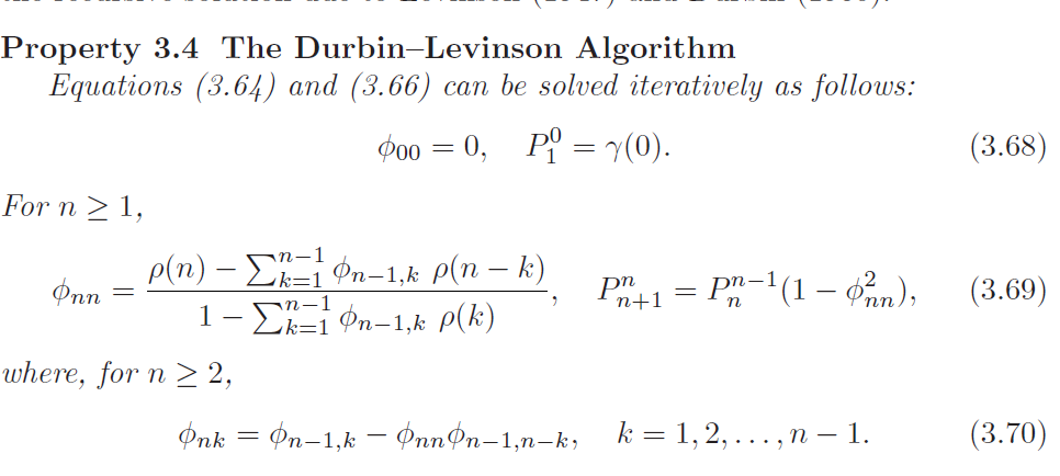
The Durbin-Levinson Algorithm
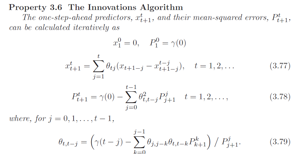
The Innovations Algorithm
Iterative Solution for the PCAF
The PCAF of a stationary process \(X_t\), can be obtained iteratively using Durbin-Levinson Algorithm as \(\phi_{nn}\) for \(n = 1, 2, ...\)
Thus, we know that the last coefficient of \(AR(p)\) model is the partial autocorrelation at lag \(p\), \(\phi_p = \phi_{pp}\).
\(m\)-step-ahead Prediction
Property 3.3 allows us to calculate the BLP of \(X_{n+m}\) for any \(m \geq 1\). Given data, the \(m\)-step-ahead predictor is:
\[X^n_{n+m} = \phi^{(m)}_{n1} X_n + \phi^{(m)}_{n2} X_{n-1} + ,..., + \phi^{(m)}_{nn} X_1\]
Where the coefficients \(\boldsymbol{\phi}^{(m)}_n\) satisfies:
\[\sum^n_{j=1} \phi^{(m)}_{nj} \gamma(k - j) = \gamma(m + k - 1), \;\; k = 1, 2, ... , n\]
The prediction equation in matrix form:
\[\Gamma_n \boldsymbol{\phi}^{(m)}_n = \boldsymbol{\gamma}^{(m)}_n\]
Where \(\boldsymbol{\gamma}^{(m)}_n = [\gamma(m), ...., \gamma(m + n - 1)]^T\) and \(\boldsymbol{\phi}^{(m)}_n = [\phi^{(m)}_{n1}, ..., \phi^{(m)}_{nn}]^T\)
The mean square \(m\)-step-ahead prediction error is:
\[P^n_{n+m} = E[X_{n + m} - X^n_{n + m}]^2 = \gamma(0) - \boldsymbol{\gamma}^{(m)^T}_n \Gamma^{-1}_n \boldsymbol{\gamma}^{(m)}_n\]
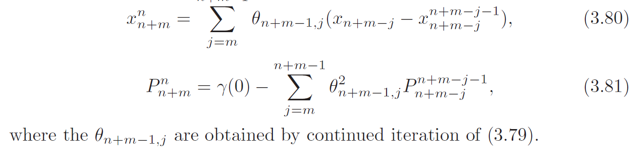
Given the data \(X_1, ..., X_n\), the innovations algorithm can be calculated successively for \(t=1\) then \(t=2\) and so on. The \(m\)-step-ahead predictor and its mean-square error based on the innovative algorithm are given by:
Forecasting \(ARMA\) Processes
The general prediction equations of BLP provides little insight into forecasting for \(ARMA\) models in general especially when \(n\) is large, we need to invert a \(n \times n\) matrix which is computationally expensive. There are a number of different ways to express these forecasts, and each aids in understanding the special structure of \(ARMA\) prediction. Throughout, we assume \(X_t\) is a causal and invertible zero-mean \(ARMA\) process, \(\phi(B)X_t = \theta(B)W_t\), where \(W_t \overset{i.i.d}{\sim} N(0, \sigma^2_w)\).
We denote the predictor of \(X_{n+m}\) based on the infinite past as:
\[\tilde{X}_{n+m} = E[X_{n+m} | X_n, ...., X_1, X_0, X_{-1}, ...]\]
In general, \(\tilde{X}_{n+m}\) is not the same as the minimum mean square error predictor \(X^n_{n+m}\), but for large samples \(\tilde{X}_{n+m}\) will provide a good approximation to it. We now write the process in invertible and causal forms:
\[X_{n+m} = \sum^\infty_{j=0} \psi_j W_{n+m-j}, \;\; \psi_0 = 1\] \[W_{n+m} = \sum^{\infty}_{j=0} \pi_j X_{n+m-j}, \;\; \pi_0 = 1\]
Then by taking the conditional expectation on infinite past, we have:
\[\tilde{X}_{n+m} = \sum^\infty_{j=0}\psi_j \tilde{W}_{n+m-j} = \sum^{\infty}_{j=m}\psi_j W_{n+m-j}\]
Since by causality and invertibility:
\[\tilde{W}_t = E[W_t | X_n, ...., X_0, ....] = E[\sum^{\infty}_{j=0} \pi_j X_{t-j} | X_n, ..., X_0, ...] = \begin{cases} 0 & t > n\\ &\\ % blank row W_{t} & t \leq n \end{cases}\]
Similarly, using the second equation we have:
\[E[W_{n+m}] = 0 = E[\sum^\infty_{j=0} \pi_j X_{n+m-j} | X_n ,...., X_0, ..] = \sum^{\infty}_{j=0}\pi_j \tilde{X}_{n+m-j} = \tilde{X}_{n+m} + \sum^{\infty}_{j=1}\pi_j \tilde{X}_{n+m-j}\]
Since \(E[X_{t} | X_n ,..., X_0, ...] = X_{t}\) for \(t \leq n\), we have:
\[\tilde{X}_{n+m} = -\sum^{\infty}_{j=1}\pi_j \tilde{X}_{n+m-j} = -\sum^{m-1}_{j=1} \pi_j \tilde{X}_{n+m-j} - \sum^{\infty}_{k=m} \pi_k X_{n + m -k}\]
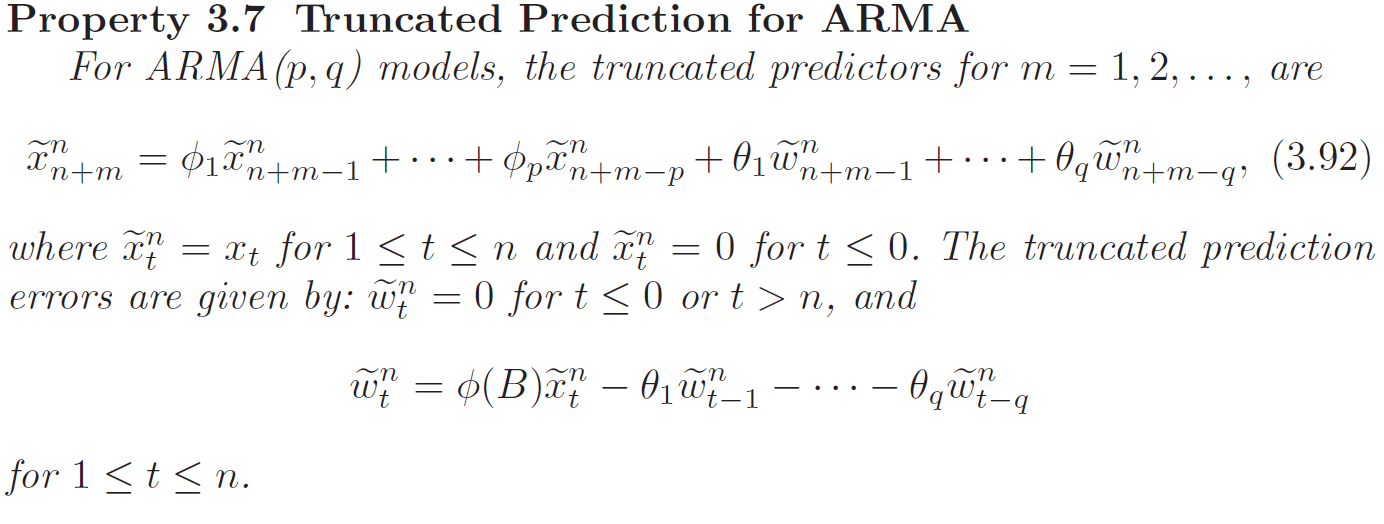
Prediction is accomplished recursively using the above equation, starting from \(m=1\), and then continuing for $m=2, 3, .. $. When \(n\) is large, we would use this by truncating, because we only observe \(X_1, X_2, ..., X_n\) but not the whole history \(X_n, ..., X_0, X_{-1}, ...\). In this case, we can truncate the above equation by setting \(\sum^{\infty}_{j=n+m} \pi_j X_{n+m-j} = 0\):
\[\tilde{X}^n_{n+m} = -\sum^{m-1}_{j=1} \pi_j \tilde{X}^n_{n+m-j} - \sum^{n + m - 1}_{k=m} \pi_k X_{n + m -k}\]
Hence, we can write the mean square prediction error as:
\[P^n_{n+m} = E[(X_{n+m} - \tilde{X}_{n+m})^2] = Var[(X_{n+m} - \tilde{X}_{n+m})^2] + E^2[X_{n+m} - \tilde{X}_{n+m}] = \sigma^2_w\sum^{m-1}_{j=0}\psi^2_j\]
Where \(X_{n+m} - \tilde{X}_{n+m} = \sum^\infty_{j=0} \psi_j W_{n+m-j} - \sum^{\infty}_{j=m}\psi_j W_{n+m-j} = \sum^{m-1}_{j=0}\psi_j W_{n+m-j}\)
The \(ARMA\) forecasts quickly settle to the mean with a constant prediction error as the forecast horizon \(m\) grows.
Integrated Models for Nonstationary Data
If \(X_t\) is a random walk, \(X_t = X_{t-1} + W_t\), then by differencing \(X_t\), we find that \(\nabla X_t = X_{t} - X_{t-1} = W_t\) is stationary. In many situations, time series can be thought of as being composed of two components:
- A nonstationary trend component.
- A zero-mean stationary component.
The intergrated ARMA (ARIMA) model is a broadening of the class of \(ARMA\) models to include differencing.
Definition: \(ARIMA\)
A process \(X_t\) is said to be \(\mathbf{ARIMA}(p, d, q)\) if:
\[\nabla^d X_t = (1 - B)^d X_t\]
is a \(ARMA(p, q)\). In general, we will write the model as:
\[\phi(B) (1 - B)^d X_t = \theta (B) W_t\]
If \(E[\nabla^d X_t] = \mu\), we write the model as:
\[\phi(B) (1 - B)^d X_t = \theta (B) W_t + \delta\]
Where:
\[\delta = \mu(1 - \phi_1 - ... - \phi_p)\]
For \(ARIMA\) model, since \(Y_t = \nabla^d X_t\) is a \(ARMA\) model, we can use the forecasting methods to obtain forecasts for \(Y_t\) which in turn leads to forecasts for \(X_t\).
If \(d=1\), given forecasts \(Y^n_{n+m}\) for \(m=1, 2, ...\), we have \[Y^n_{n+m} = X^n_{n+m} - X^n_{n+m-1}\] \[\implies X^n_{n+m} = X^n_{n+m-1} + Y^n_{n+m}\] With initial condition: \[X^n_{n+1} = X_{n} + Y^n_{n+1}\] Since: \[X^n_{n} = X_n\]
For \(ARIMA\) models, the mean-squared error can be approximated by:
\[P^n_{n+m} = \sigma^2_w \sum^{m-1}_{j=0} {\psi^*_j}^2\]
Where \(\psi^*_j\) is the coefficient of \(z^j\) in \(\psi^*(z) = \frac{\theta(z)}{\phi(z)(1 - z)^d}\)
EMA
The Exponentially Weighted Moving Average(EWMA) is defined as a \(ARIMA(0, 1, 1)\) model:
\[X_t = X_{t-1} + W_t- \lambda W_{t-1}\]
Where \(|\lambda| < 1\) for \(t = 1, 2, ...\) and \(X_0 = 0\).