real-analysis-4

Posted on 2022-01-06 Edited on 2022-06-17 In Background Views:

Symbols count in article: 20k Reading time ≈ 18 mins.

Real Analysis (4)

Sequences and Series of Functions [1]

Uniform Convergence of a Seuqence of Functions

Definition 6.2.1: Pointwise Convergence

For each $n \in \mathbb{N}$, let $f_n$ be a function defined on a set $A \subseteq \mathbb{R}$. The sequence $(f_n)$ of functions converges pointwise on $A$ to a function $f$ if, for all $x \in A$, the sequence of real numbers $f_{n} (x)$ converges to $f(x)$.

In this case, we write $f_n \rightarrow f$, $\lim_{n \rightarrow \infty} f_n = f$ or $\lim_{n \rightarrow \infty} f_n(x) = f(x)$.

Definition 6.2.1B: Pointwise Convergence

Let $(f_n)$ be a sequence of functions defined on a set $A \subseteq \mathbb{R}$. Then, $(f_n)$ convergence pointwise on $A$ to a limit function $f$ defined on $A$ if, for every $\epsilon > 0$ and $x \in A$, there exists an $N \in \mathbb{N}$ (perhaps depends on $x$) such that $|f_{n} (x) - f(x) | < \epsilon$ whenever $n \geq N$.

Definition 6.2.3: Uniform Convergence (Stronger than Pointwise)

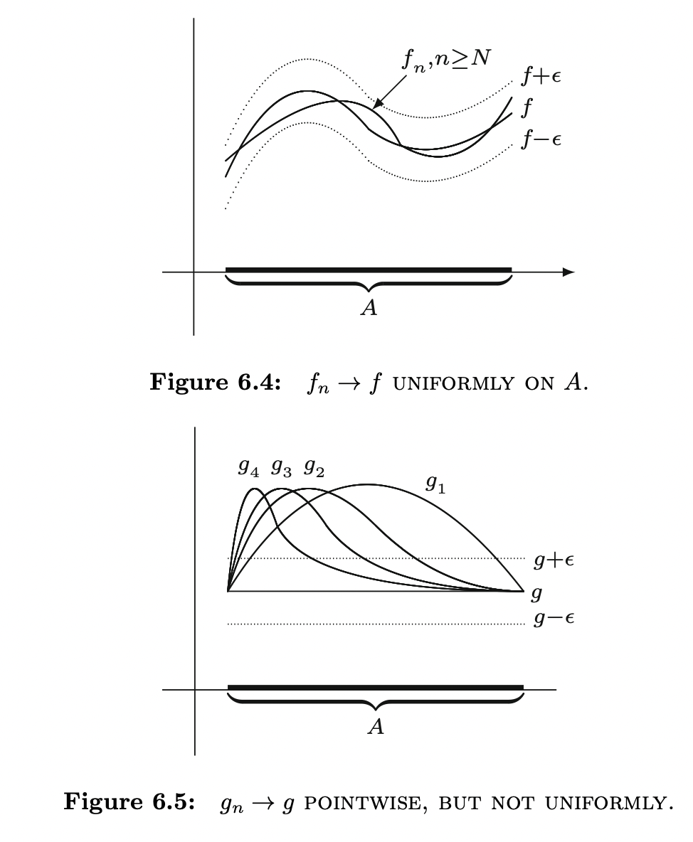
Let $(f_n)$ be a sequence of functions defined on a set $A \subseteq \mathbb{R}$. Then, $(f_n)$ convergence uniformly on $A$ to a limit function $f$ defined on $A$ if, for every $\epsilon > 0$, there exists an $N \in \mathbb{N}$ such that $|f_{n} (x) - f(x) | < \epsilon$ whenever $n \geq N$ and $x \in A$.

Similar to uniform continuous, this is a stronger, which involves finding $N \in \mathbb{N}$ for a given $\epsilon > 0$ for all $x \in A$.

Graphically speaking, the uniform convergence of $f_n$ to a limit $f$ on a set $A$ can be seen as there exists a point in the sequence after which each $f_n$ is completely contained in the $\epsilon$-strip.

Theorem 6.2.5: Cauchy Criterion for Uniform Convergence

A sequence of functions $(f_n)$ defined on a set $A \subseteq \mathbb{R}$ converges uniformly on $A$ if and only if for every $\epsilon > 0$ there exists an $N \in \mathbb{N}$ such that $|f_n(x) - f_m(x)| < \epsilon$ whenever $m, n \geq N$ for all $x \in A$.

Theorem 6.2.6: Continuous Limit Theorem

Let $(f_n)$ be a sequence of functions defined on $A \subseteq \mathbb{R}$ that converges uniformly on $A$ to a function $f$. If each $f_n$ is continuous at $c \in A$, then $f$ is continuous at $c$.

Uniform Convergence and Differentiation

Theorem 6.3.1: Differentiable Limit Theorem

Let $f_n \rightarrow f$ pointwise on the closed interval $[a, b]$, and assume that each $f_n$ is differentiable. If $(f^{\prime}(c))$ converges uniformly on $[a, b]$ to a function $g$, then the function $f$ is differentiable and $f^{\prime} = g$.

Theorem 6.3.2

Let $(f_n)$ be a sequence of differentiable functions defined on the closed interval $[a, b]$, and assume $(f^{\prime}_n)$ converges uniformly on $[a, b]$. If there exists a point $x_0 \in [a, b]$, where $f_{n} (x_0)$ is convergent, then $(f_n)$ converges uniformly on $[a, b]$.

Theorem 6.3.3: Combine Theorem 6.3.1 and 6.3.2

Let $(f_n)$ be a sequence of differentiable functions defined on the closed interval $[a, b]$, and assume $(f^{\prime}_n)$ converges uniformly on $[a, b]$ to a function $g$ on $[a, b]$. If there exists a point $x_0 \in [a, b]$, where $f_{n} (x_0)$ is convergent, then $(f_n)$ converges uniformly on $[a, b]$. Moreover, the limit function $f = \lim_{n\rightarrow \infty} f_n$ is differentiable and satisfies $f^{\prime} = g$.

Series of Functions

Definition 6.4.1: Pointwise Convergence and Uniform Convergence of Series of Functions

For each $n \in \mathbb{N}$, let $f_n$ and $f$ be functions defined on a set $A \subseteq \mathbb{R}$. The infinite series:

\[\sum^{\infty}_{n=1} f_n = f_1 + f_2 + .... \]

converges pointwise on $A$ to $f$ if the sequence $s_k$ of partial sums defined by:

\[s_k = f_1 + f_2 + ... + f_k\]

converges pointwise to $f$. The series converges uniformly on $A$ to $f$ if the sequence $s_k$ converges uniformly on $A$ to $f$. In either case, we can write:

\[f = \sum^{\infty}_{n=1} f_n\]

\[f(x) = \sum^{\infty}_{n=1} f_n(x)\]

Theorem 6.4.2: Term-by-Term Continuity Theorem

Let $f_n$ be continuous functions defined on a set $A \subseteq \mathbb{R}$, and assume $\sum^{\infty}_{m=1} f_n$ converges uniformly on $A$ to a function $f$. Then $f$ is continuous on $A$.

Theorem 6.4.3: Term-by-Term Differentiability Theorem

Let $f_n$ be differentiable functions defined on an interval $A$, and assume $\sum^{\infty}_{n=1} f^{\prime}_n$ converges uniformly to a limit function $g$ on $A$. If there exists a point $x_0 \in [a, b]$ where $\sum^{\infty}_{n=1} f_n (x_0)$ converges, then the series $\sum^{\infty}_{n=1} f_n$ converges uniformly to a differentiable function $f$ satisfying $f^{\prime} = g$ on $A$.

Theorem 6.4.4: Cauchy Criterion for Uniform Convergence of Series

A series $\sum^{\infty}_{n=1} f_n$ converges uniformly on $A \subseteq \mathbb{R}$ if and only if for every $\epsilon > 0$ there exists an $N \in \mathbb{N}$ s.t

\[|f_{m+1} (x) + f_{m+2} (x) + ... + f_{n} (x) | < \epsilon\]

whenever $n > m \geq N$ and $x \in A$

Corollary 6.4.5: Weierstrass M-Test

For each $n \in \mathbb{N}$, let $f_n$ be a function defined on a set $A \subseteq \mathbb{R}$, and let $M_n > 0$ be a real number satisfying:

\[|f_n(x)| \leq M_n\]

for all $x \in A$. If $\sum^{\infty}_{n=1} M_n$ converges, then $\sum^{\infty}_{n=1} f_n$ converges uniformly on $A$.

Power Series

\[f(x) = \sum^{\infty}_{n=0} a_n x^n = a_0 + a_1x + a_2x^2 + a_3 x^3 + ...\]

Theorem 6.5.1

If a power series $\sum^{\infty}_{n=0} a_n x^n$ converges at some point $x_0 \in \mathbb{R}$, then it converges absolutely for any $x$ satisfying $|x| < |x_0|$.

Theorem 6.5.2

If a power series $\sum^{\infty}_{n=0} a_n x^n$ converges absolutely at a point $x_0$, then it converges uniformly on the closed interval $[-c, c]$, where $c=|x_0|$.

Lemma 6.5.3: Abel's Lemma

Let $b_n$ satisfy $b_1 \geq b_2 \geq b_3 \geq .... \geq 0$, and let $\sum^{\infty}_{n=1} a_n$ be a series for which the partial sums are bounded. In other words, assume there exists $A > 0$ s.t

\[|a_1 + a_2 + ... + a_n| \leq A\]

for all $n \in \mathbb{N}$. Then for all $n \in \mathbb{N}$,

$$|a_1b_1 + a_2b_2 + .... + a_nb_n|

Theorem 6.5.4: Abel's Theorem

Let $g(x) = \sum^{\infty}_{n=0} a_nx^n$ be a power series that converges at the point $x = R > 0$. Then the series converges uniformly on the interval $[0, R]$. A similar result holds if the series converges at $x = -R$.

Theorem 6.5.5

If a power series converges pointwise on the set $A \subseteq \mathbb{R}$, then it converges uniformly on any compact set $K \subseteq A$.

Theorem 6.5.6

If $\sum^{\infty}_{n=0}a_n x^n$ converges for all $x \in (-R, R)$, then the differentiated series $\sum^{\infty}_{n=1} na_n x^{n-1}$ converges at each $x\in (-R, R)$ as well. Consequently, the convergence is unifrom on compact sets contained in $(-R, R)$.

Theorem 6.5.7

Assume

\[f(x) = \sum^{\infty}_{n=0} a_n x^n\]

converges on an interval $A \subseteq \mathbb{R}$. The function $f$ is continuous on $A$ and differentiable on any open interval $(-R, R) \subseteq A$. The derivative is given by:

\[f^{\prime} (x) = \sum^{\infty}_{n=1} na_nx^{n-1}\]

Moreover, $f$ is infinitely differentiable on $(-R, R)$, and the successive derivatives can be obtained via term-by-term differentiation of the appropriate series.

Taylor Series

Given an infinitely differentiable function $f$ defined on some interval centered at zero, the idea is to assume that $f$ has a power series expansion and deduce what the coefficients must be. (Not every infinitely differentiable function can be represented by its taylor series)

Theorem 6.6.2: Taylor's Formula Centered at Zero (Maclaurin Series)

Let

\[f(x) = a_0 + a_1x + a_2x^2 + ...\]

be defined on some nontrivial interval centered at zero. Then:

\[a_n = \frac{f^{(n)}(0)}{n!}\]

Where $f^{(n)}(0)$ is the $n$th derivative of $f$ evaluate at $0$.

This formula assumes that the function $f$ has a power series representation.

Theorem 6.6.3: Lagrange's Remainder Theorem

Let $f$ be differentiable $N + 1$ times on $(-R, R)$, define $a_n = \frac{f^{n} (0)}{n!}$ for $n=0, 1, ... , N$, and let:

\[S_N(x) = a_0 + a_1 x + a_2 x^2 + ... + a_N x^N\]

Given $x \neq 0$ in $(-R, R)$, there exists a point $c$ satisfying $|c| < |x|$ where the error function $E_N(x) = f(x) - S_N (x)$ satisfies:

\[E_N(x) = \frac{f^{(N+1)} (c)}{(N+1)!} x^{N+1}\]

Definition 6.6.7: Taylor Series Centered at $a \neq 0$

If $f$ is defined in some neighborhood of $a \in \mathbb{R}$ and infinitely differentiable at $a$, then the Taylor series expansion around $a$ takes the form:

\[\sum^{\infty}_{n=0}c_n (x - a)^n\]

where $c_n = \frac{f^{(n)} (a)}{n!}$

The Weierstrass Approximation Theorem

Theorem 6.7.1: Weierstrass Approximation Theorem

Let $f: [a, b] \rightarrow \mathbb{R}$ be continuous. Given $\epsilon > 0$, there exists a polynomial $p(x)$ satisfying:

\[|f(x) - p(x) | < \epsilon\]

for all $x \in [a, b]$.

In other words, every continuous function on a closed interval can be uniformly approximated by a polynomial.

Definition 6.7.2: Polygonal

A continuous function $\phi: [a, b] \rightarrow \mathbb{R}$ is polygonal if there is a partition:

\[a = x_0 < x_1 < x_2 < .... < x_n = b\]

of $[a, b]$ such that $\phi$ is linear on each subinterval $[x_{i-1}, x_i]]$ where $i=1, ..., n$

Theorem 6.7.3

Let $f: [a, b] \rightarrow \mathbb{R}$ be continuous. Given $\epsilon > 0$, there exists a polygonal function $\phi$ satisfying:

\[|f(x) - \phi(x) | < \epsilon\]

The Riemann Integral

The Definition of the Riemann Integral

Throughout this section, it is assumed that we are working with a bounded function $f$ on a closed interval $[a, b]$, meaning that there exists an $M > 0$ s.t $|f(x)| \leq M, \; \forall x \in [a, b]$

Definition 7.2.1: Partition, Lower Sum, Upper Sum

A partition $P$ of $[a, b]$ is a finite set of points from $[a, b]$ that includes both $a$ and $b$. A partition $P = \{x_0, ...., x_n\}$ is listed in increasing order:

\[a=x_0 < x_1 < x_2 < ... < x_n = b\]

For each subinterval $[x_{k-1}, x_k]$ of $P$, let:

\[m_k = \inf\{f(x): x \in [x_{k-1}, x_k]\}\]

and

\[M_k = \sup\{f(x): x\in[x_{k-1}, x_k]\}\]

Since the function is bounded, the supreme and infimum always exists.

The lower sum of $f$ w.r.t $P$ is given by:

\[L(f, P) = \sum^{n}_{k=1} m_k (x_k - x_{k-1})\]

The upper sum of $f$ w.r.t $P$ is given by:

\[U(f, P) = \sum^{n}_{k=1} M_k (x_k - x_{k-1})\]

For a particular partition $P$, it is clear that:

\[U(f, P) \geq L(f, P)\]

A partition $Q$ is a refinement of a partition $P$ if $Q$ contains all of the points of $P$ if $Q$ contains all of the points of $P$; that is, if $P \in Q$.

Lemma 7.2.3

If $P \subseteq Q$, then $L(f, P) \leq L(f, Q)$, and $U(f, P) \geq U(f, Q)$.

Lemma 7.2.4

If $P_1, P_2$ are any two partitions of $[a, b]$, then $L(f, P_1) \leq U(f, P_2)$.

We can think of upper sum as an overestimate for the value of the integral and a lower sum as an underestimate. As the partitions get more refined, the upper sums get potentially smaller while the lower sums get potentially larger.

Definition 7.2.5: Upper Integral, Lower Integral

Let $\mathbf{P}$ be the collection of all possible partitions of the interval $[a, b]$. The upper integral of $f$ is defined to be:

\[U(f) = \inf\{U(f, P): P \in \mathbf{P}\}\]

In a similar way, define the lower integral of $f$ by:

\[L(f) = \sup\{L(f, P): P\in\mathbf{P}\}\]

Lemma 7.2.6

For any bounded function $f$ on $[a, b]$, it is always the case that $U(f) \geq L(f)$.

Definition 7.2.7: Riemann Integrability

A bounded function $f$ defined on the interval $[a, b]$ is Riemann-integrable if $U(f) = L(f)$. In this case, we define $\int^{b}_{a} f$ or $\int^{a}_{b} f(x) dx$ to be this common value, namely:

\[\int^b_{a} f = U(f) = L(f)\]

Criteria for Integrability

Theorem 7.2.8: Integrability Criterion

A bounded function $f$ is integrable on $[a, b]$ if and only if, for every $\epsilon > 0$, there exists a partition $P_{\epsilon}$ of $[a, b]$ s.t

\[U(f, P_\epsilon) - L(f, P_{\epsilon}) < \epsilon\]

Theorem 7.2.9

If $f$ is continuous on $[a, b]$, then it is integrable.

Theorem 7.3.2

If $f: [a, b] \rightarrow \mathbb{R}$ is bounded, and $f$ is integrable on $[c, b]$ for all $c \in (a, b)$, then $f$ is integrable on $[a, b]$. An analogous result holds at the other end point.

Properties of the Integral

Theorem 7.4.1

Assume $f: [a, b] \rightarrow \mathbb{R}$ is bounded, and let $c \in (a, b)$. Then, $f$ is integrable on $[a, b]$ if and only if $f$ is integrable on $[a, c]$ and $[c, b]$. In this case, we have:

\[\int^{b}_{a} f = \int^{c}_{a} f + \int^{b}_{c} f\]

Theorem 7.4.2

Assume $f, g$ are integrable functions on the interval $[a, b]$.

The function $f + g$ is integrable on $[a, b]$ with $\int^{b}_{a} (f + g) = \int^{b}_{a} f + \int^{b}_{a} g$.
For $k \in \mathbb{R}$, the function $kf$ is integrable with $\int^{b}_{a} kf = k \int^{b}_{a} f$.
If $m \leq f(x) \leq M$ on $[a, b]$, then $m(b - a) \leq \int^{b}_{a} f \leq M (b - a)$.
If $f(x) \leq g(x)$ on $[a, b]$, then $\int^{b}_{a} f \leq \int^b_a g$
The function $|f|$ is integrable and $|\int^{b}_{a} f| \leq \int^{b}_{a} |f|$

Definition 7.4.3

If $f$ is integrable on the interval $[a, b]$, define:

\[\int^a_{b} f = - \int^b_a f\]

Also, for $c \in [a, b]$, definte:

\[\int^c_c f = 0\]

Theorem 7.4.4: Integrable Limit Theorem

Assume that $f_n \rightarrow f$ uniformly on $[a, b]$ and that each $f_n$ is integrable. Then $f$ is integrable and:

\[\lim_{n \rightarrow \infty} f_n = \int^b_{a} f\]

The Fundamental Theorem of Calculus

Theorem 7.5.1: Fundamental Theorem of Calculus

If $f: [a, b] \rightarrow \mathbb{R}$ is integrable, and $\mathbb{F}: [a, b] \rightarrow \mathbb{R}$ satisfies $F^{\prime} (x) = f(x) \;\; \forall x \in [a, b]$ satisfies $F^{\prime} (x) = f(x), \; \forall x \in [a, b]$, then:

\[\int^b_a f = F(b) - F(a)\]
Let $g: [a, b] \rightarrow \mathbb{R}$ be integrable, and for $x \in [a, b]$, define:

\[G(x) = \int^x_a g\]

Then $G$ is continuous on $[a, b]$. If $g$ is continuous at some point $c \in [a, b]$, then $G$ is differentiable at $c$ and $G^{\prime}(c) = g(c)$

\[G^{\prime}(x) = \frac{d}{dx} \int^x_a g = g(x)\]

Definition 7.6.1: Measure Zero

A set $A \subseteq \mathbb{R}$ has measure zero if, for all $\epsilon > 0$, there exists a countable collection of open intervals $O_n$ with the property that $A$ is contained in the union of all of the intervals $O_n$ and the sum of the lengths of all of the intervals is less than or equal to $\epsilon$. More precisely, if $|O_n|$ refers to the length of the interval $O_n$, then we have:

\[A \subseteq \bigcup^{\infty}_{n=1} O_n\]

and

\[\sum^{\infty}_{n=1} | O_n | \leq \epsilon\]

Consider a finite set $A = \{a_1, ..., a_n\}$. To show that $A$ has measure zero, let $\epsilon > 0$ be arbitrary. For each $1 \leq n < N$, construct the interval: \[G_n = (a_n - \frac{\epsilon}{2N}, a_n + \frac{\epsilon}{2N})\]

Clearly, $A$ is contained in the union of these intervals, and \[\sum^N_{n=1} | G_n | = \sum^N_{n=1}\frac{\epsilon}{N} = \epsilon\]

Definition 7.6.3: $\alpha$-Continuity

Let $f$ be defined on $[a, b]$, and let $\alpha > 0$. The function $f$ is $\alpha$-continuous at $x \in [a, b]$ if there exists $\delta > 0$ s.t for all $y, z \in (x - \delta, x + \delta)$, it follows that $|f(y) - f(z)| < \alpha$.

Let $f$ be a bounded function on $[a, b]$, for each $\alpha > 0$, defined $D^{\alpha}$ to be the set of points in $[a, b]$, where the function $f$ fails to be $\alpha$-continuous;

Definition 7.6.4: Uniformly $\alpha$-continuous

A function $f: A \rightarrow \mathbb{R}$ is uniformly $\alpha$-continuous on $A$, if there exists a $\delta > 0$ s.t whenever $x$ and $y$ are points in $A$ satisfying $|x - y| < \delta$, it follows that $|f(x) - f(y)| < \alpha$..

Theorem 7.6.5 Lebesgue's Theorem

Let $f$ be a bounded function defined on the interval $[a, b]$. Then, $f$ is Riemann-integrable if and only if the set of points where $f$ is not continuous has measure zero.

Definition 8.4.3: Improper Riemann Integrals

Assume $f$ is defined on $[a, \infty)$ and integrable on every interval of the form $[a, b]$. Then define $\int^{\infty}_{a} f$ to be:

\[\lim_{b \rightarrow \infty} \int^{b}_{a} f\]

provided the limit exists, in this case we say that the improper integral $\int^{\infty}_a f$ converges.

Interchange of Limits [2]

Theorem 8.2.4

Let $(f_n)$ be a sequence of functions be defined on $[a, b] \in \mathbb{R}$ and suppose that $(f_n)$ converges uniformly on $[a, b]$ to $f$. Then $f \in \mathbb{R}$ and:

\[\int^{a}_{b} f = \lim_{n \rightarrow \infty} \int^b_a f_n\]

We can switch the integral and the limit.

Theorem 8.2.5: Bounded Convergence Theorem

Let $(f_n)$ be a sequence defined on $\mathbb{R}[a, b]$ that converges on $[a, b]$ to a function $f \in \mathbb{R} [a, b]$. Suppose also that there exists a $B > 0$ s.t $|f_n(x)| \leq B, \; \forall x \in [a, b]$, $n \in \mathbb{N}$. Then:

\[\int^{a}_{b} f = \lim_{n \rightarrow \infty} \int^b_a f_n\]

Theorem 8.2.6: Dini's Theorem

Suppose that $(f_n)$ is a monotone sequence of continuous functions on $I:=[a, b]$ that converges on $I$ to a continuous function $f$. Then the convergence of the sequence is uniform.

The Exponential Function

Theorem 8.3.1:

There exists a function $E: \mathbb{R} \rightarrow \mathbb{R}$ s.t:

$E^{\prime} (x) = E(x)$
$E(0) = 1$

Partial Proof of Theorem 8.3.1

We define a sequence $(E_n)$ of continuous functions as follows:

$E_{1} (x) := 1 + x$
$E_{n + 1} (x) := 1 + \int^x_0 E_n(t) dt$

for all $n \in \mathbb{N}, x \in \mathbb{R}$, we can also show that:

\[E_{n} (x) = 1 + \frac{x}{1!} + \frac{x^2}{2!} + ... + \frac{x^n}{n!}\]

We can show that the limiting function $E = \lim_{n\rightarrow \infty}$ exists and satisfies all two points of theorem 8.3.1.

Corollary 8.3.2

The function $E$ has a derivative of every order and $E^(n) (x) = E(x), \; \forall n \in \mathbb{N}, x \in \mathbb{R}$.

Corollary 8.3.3

If $x > 0$, then $1 + x < E(x)$

Theorem 8.3.4

The function $E: \mathbb{R} \rightarrow \mathbb{R}$ that satisfies theorem 8.3.1 (i) and (ii) is unique.

Definition 8.3.5

The unique function $E: \mathbb{R} \rightarrow \mathbb{R}$, such that $E^{\prime} (x) = E(x)$ for all $x \in \mathbb{R}$ and $E(0) = 1$ is called the exponential function. The number $e := E(1)$ is called Euler's number:

\[\exp(x) := E(x)\]

\[e^x := E(x)\]

for $x \in \mathbb{R}$

Theorem 8.3.6

The exponential function satisfies the following properties:

$E(x) \neq 0, \; \forall x \in \mathbb{R}$
$E(x + y) = E(x)E(y), \; \forall x, y \in \mathbb{R}$
$E(r) = e^r, \;\forall r \in \mathbb{Q}$

Theorem 8.3.7

The exponential function $E$ is strictly increasing on $\mathbb{R}$ and has range equal to $y \in \mathbb{R}: y > 0$. Further, we have:

$\lim_{x \rightarrow \infty} E(x) = 0$
$\lim_{x \rightarrow \infty} E(x) = \infty$

The Logarithm Function

Definition 8.3.8: Logarithm Function

The function inverse to $E: \mathbb{R} \rightarrow \mathbb{R}$ is called the logarithm (natural logarithm) denoted by $L$ or by $\ln$.

Since they are inverse, we have:

\[(L \circ E) (x) = x, \; \forall x \in \mathbb{R}\]

and

\[(E \circ L) (y) = y, \; \forall y \in \mathbb{R}, y > 0\]

Theorem 8.3.9

The logarithm is a strictly increasing function $L$ with doman $x \in \mathbb{R}: x > 0$ and range $\mathbb{R}$. The derivative of $L$ is given by:

$L^{\prime} (x) = \frac{1}{x}$
$L(xy) = L(x) L(y)$
$L(1) = 0, L(e) = 1$
$L(x^r) = rL(x), \; \forall r \in \mathbb{Q}$
$\lim_{x \rightarrow 0^+} L(x) = -\infty$ and $\lim_{x \rightarrow \infty} L(x) = \infty$

Power Function

Definition 8.3.10: Power Function

If $\alpha \in \mathbb{R}$ and $x > 0$, the number $x^\alpha$ is defined to be

\[x^\alpha := e^{\alpha \ln x} = E(\alpha L(x))\]

The function $x \rightarrow x^\alpha$ for $x > 0$ is called the power function with exponent $\alpha$.

Theorem 8.3.11

If $\alpha \in \mathbb{R}$ and $x, y$ belong to $(0, \infty)$, then:

$1^\alpha = 1$
$x^\alpha > 0$
$(xy)^\alpha = x^\alpha y^\alpha$
$(\frac{x}{y})^{\alpha} = \frac{x^\alpha}{y^\alpha}$

Theorem 8.3.12

If $\alpha, \beta \in \mathbb{R}$ and $x \in (0, \infty)$, then:

$x^{\alpha + \beta} = x^{\alpha} + x^{\beta}$
$(x^\alpha)^\beta = x^{\alpha\beta} = (x^{\beta})^\alpha$
$x^{-\alpha} = \frac{1}{x^\alpha}$
If $\alpha < \beta$, then $x^\alpha < x^\beta$ for $x > 1$

Theorem 8.3.13

Let $\alpha \in \mathbb{R}$. Then the function $x \rightarrow x^\alpha$ on $(0, \infty)$ to $\mathbb{R}$ is continuous and differentiable, and

\[D x^\alpha = \alpha x^{\alpha - 1}\]

If $\alpha > 0$ the power function is strictly increasing, if $\alpha < 0$, the power function is strictly decreasing.

Function $\log_a$

if $a > 0$, $a \neq 1$, it is sometimes useful to define the function $\log_a$

Definition 8.3.14

Let $a > 0, a \neq 1$. We define:

\[\log_a (x) := \frac{\ln x}{\ln a}\]

for $x \in (0, \infty)$

This is called logarithm of $x$ to the base $a$.

The Trigonometric Function

Theorem 8.4.1

There exist functions $C: \mathbb{R} \rightarrow \mathbb{R}$ and $S: \mathbb{R} \rightarrow \mathbb{R}$ such that:

$C^{\prime\prime} (x) = - C(x)$ and $S^{\prime\prime} (x) = - S(x)$ for all $S: \mathbb{R} \rightarrow \mathbb{R}$.
$C(0) = 1, C^{\prime} (0)$, and $S(0) = 0, S^{\prime} (0) = 1$

Partial Proof of Theorem 8.4.1

Define the sequences $(C_n), (S_n)$ of continuous functions inductively as:

$C_1 (x) := 1, \; S_1 (x) := x$
$S_n(x) := \int^x_0 C_n(t) dt$
$C_{n+1} (x) := 1 - \int^x_0 S_n(t) dt$

for all $n \in \mathbb{N}, x \in \mathbb{R}$. By induction, we have:

\[C_{n+1} (x) = 1 - \frac{x^2}{2!} + \frac{x^4}{4!} - ... + (-1)^n \frac{x^{2n}}{(2n)!}\] \[S_{n+1} (x) = x - \frac{x^3}{3!} + \frac{x^5}{t!} - .... + (-1)^n \frac{x^{2n+1}}{(2n+1)!}\]

Then the sequences converges uniformly to some function $C, S$ that satisfies all the properties of theorem 8.4.1.

Corollary 8.4.2

If $C, S$ are the functions in theorem 8.4.1, then:

$C^{\prime} (x) = -S(x)$ and $S^{\prime} (x) = C(x)$ for all $x \in \mathbb{R}$.

Moreover, these functions have derivatives of all orders.

Corollary 8.4.3

The functions $C, S$ satisfy the pythagorean identity:

$(C(x))^2 + (S(x))^2 = 1$

Theorem 8.4.4

The function $C, S$ satisfying properties of theorem 8.4.1 are unique.

Definition 8.4.5

The unique functions $C: \mathbb{R} \rightarrow \mathbb{R}$, $S: \mathbb{R} \rightarrow \mathbb{R}$ satisfying properties in theorem 8.4.1 are called cosine function and sine function:

\[\cos x := C(x)\] \[\sin x := S(x)\]

Theorem 8.4.6

If $f: \mathbb{R} \rightarrow \mathbb{R}$ is such that

\[f^{\prime\prime} (x) = -f(x), \;\; \forall x \in \mathbb{R}\]

then there exist real numbers $\alpha, \beta$ s.t

\[f(x) = \alpha C(x) + \beta S(x)\]

Theorem 8.4.7:

The function $C$ is even and $S$ is odd in the sense that:

$C(-x) = C(x)$ and $S(-x) = - S(x)$

If $x, y \in \mathbb{R}$, then we have the addition formula:

\[C(x + y) = C(x) C(y) - S(x)S(y)\] \[S(x + y) = S(x)C(y) + C(x)S(y)\]

Ref

[1] Understanding Analysis by Stephen Abbott

[2] Introduction to Real Analysis by G.Bartle, R.Sherbert