Rigorous Probability (1)

Preliminaries

For \(x, y \in \mathbb{\bar{R}} := \mathbb{R} \cup \{-\infty, \infty\}\), we agree on the following notation:

1. \(x \vee y = \max (x, y)\)
2. \(x \wedge y = \min(x, y)\)
3. \(x^+ = \max(x, 0)\)
4. \(x^- = \max(-x, 0)\)
5. \(|x| = \max(x, -x) = x^- + x^+\)
6. \(sign(x) = I_{x > 0} - I_{x < 0}\)

Class of Sets

Let \(\Omega \neq \emptyset\), let \(\mathbf{A} \subseteq 2^{\Omega}\) (set of all possible subsets of \(\Omega\)) be a class of subsets of \(\Omega\).

Definition 1.1: \(\cap\)-closed, \(\sigma-\cap\)-closed, \(\cup\)-closed, \(\sigma-\cup\)-closed, \(/\)-closed, \(A^c\)-closed

A class of sets \(\mathbf{A} \in 2^{\Omega}\) is called:

• \(\cap\)-closed (closed under intersections) or \(\pi\)-system if \(A \cap B \in \mathbf{A}\), whenever \(A, B \in \mathbf{A}\).
• \(\sigma-\cap-\)closed (closed under countable intersections) if \(\bigcap^{\infty}_{n=1}A_n \in \mathbf{A}\) for any choice of countably (finite or countably infinite) many sets \(A_1, A_2, ...., \in \mathbf{A}\).
• \(\cup-\)closed (closed under unions) if \(A \cup B \in \mathbf{A}\), whenever \(A, B \in \mathbf{A}\).
• \(\sigma-\cup-\)closed (closed under countable unions) if \(\bigcup^{\infty}_{n=1}A_n \in \mathbf{A}\) for any choice of countably (finite or countably infinite) many sets \(A_1, A_2, ...., \in \mathbf{A}\).
• \(/-\)closed (closed under differences) if \(A / B \in \mathbf{A}\), whenever \(A, B \in \mathbf{A}\).
• closed under complements if \(A^c := \Omega / A \in A\) for any set \(A \in \mathbf{A}\).

Definition 1.2: \(\sigma-\)algebra

A class of sets \(A \subseteq 2\) is called a \(\sigma\)-algebra if it fulfills the following three properties:

1. \(\Omega \in \mathbf{A}\).
2. \(\mathbf{A}\) is closed under complements.
3. \(\mathbf{A}\) is closed under countable unions.

If \(\mathbf{A}\) is \(\sigma\)-algebra, we also have:

• \(\mathbf{A}\) is \(\cup\)-closed \(\Longleftrightarrow\) \(\mathbf{A}\) is \(\cap\)-closed.
• \(\mathbf{A}\) is \(\sigma-\cup\)-closed \(\Longleftrightarrow\) \(\mathbf{A}\) is \(\sigma-\cap\)-closed
• \(\mathbf{A}\) is closed under differences
• Any countable union of sets in \(\mathbf{A}\) cna be expressed as a countable disjoint union of sets in \(\mathbf{A}\)

Definition 1.6: Algebra

A class of sets \(\mathbf{A} \subseteq 2^{\pi}\) is called an algebra if the following three conditions are fulfilled:

1. \(\Omega \in \mathbf{A}\).
2. \(\mathbf{A}\) is \(/\)-closed.
3. \(\mathbf{A}\) is \(\cup\)-closed.

If \(\mathbf{A}\) is Algebra, we also have:

1. \(\mathbf{A}\) is closed under complements.
2. \(\mathbf{A}\) is closed under intersections.

Definition 1.8: Ring

A class of sets \(\mathbf{A} \in 2^{\Omega}\) is called a ring if the following three conditions hold:

1. \(\emptyset \in \mathbf{A}\).
2. \(\mathbf{A}\) is \(/\)-closed.
3. \(\mathbf{A}\) is \(\cup\)-closed.

A ring is called \(\sigma\)-ring if it is also \(\sigma-\cup\)-closed.

Definition 1.9: Semiring

A class of sets \(\mathbf{A} \subseteq 2^\Omega\) is called a semiring if

1. \(\emptyset \in \mathbf{A}\).
2. for any two sets \(A, B \in \mathbf{A}\), \(B / A\) is a finite union of mutually disjoint sets in \(\mathbf{A}\).
3. \(\mathbf{A}\) is \(\cap\)-closed.

Definition 1.10: \(\lambda\)-system

A class of sets \(\mathbf{A} \subseteq 2^\Omega\) is called a \(\lambda\)-system if:

1. \(\Omega \in \mathbf{A}\).
2. For any two sets \(A, B \in \mathbf{A}\) with \(A \subseteq B\), the difference set \(B / A \in \mathbf{A}\).
3. \(\uplus^{\infty}_{n=1} A_n \in A\) for any choice of countably many pairwise disjoint sets \(A_1, A_2, .... \in \mathbf{A}\).

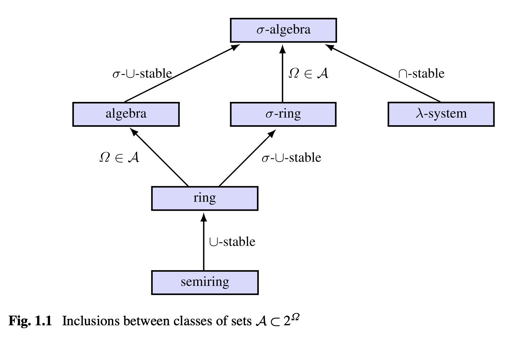
Theorem 1.12: Relations Between Classes of Sets

1. Every \(\sigma\)-algebra is also a \(\lambda\)-system, an algebra, and a \(\sigma\)-ring.
2. Every \(\sigma\)-ring is a ring, and every ring is a semiring.
3. Every algebra is a ring. An algebra on a finite set \(\Omega\) is a \(\sigma\)-algebra.

Definition 1.13: Limit Inferior and Limit Superior of Sequence and Sets

The limit inferior of a sequence \((a_n)\) is defined as:

\[\lim\inf_n a_n = \lim_{n \rightarrow \infty} \inf_{k \geq n} a_n\]

and the limit superior of the sequence is defined as:

\[\lim\sup_n a_n = \lim_{n \rightarrow \infty} \inf_{k \geq n} a_n\]

Furthermore, \(\lim_n a_n\) exists IFF \(\lim\sup_n a_n = \lim \inf_n a_n\)

Given subsets \(A_1, A_2, ... \in 2^{\Omega}\), we define infinitely many:

\[A^* := \lim\sup_n A_n = \lim_{n \rightarrow \infty} \bigcup^{\infty}_{k=n} A_n = \bigcap^{\infty}_{n=1}\bigcup^{\infty}_{k=n} A_k\]

\[w \in \bigcap^{\infty}_{n=1}\bigcup^{\infty}_{k=n} A_k \implies \forall N \geq 1, \exists k \geq N \text{ s.t } w \in A_n\]

This is equivalently saying that:

\[\{x: \text{ $x$ in infinitely many $A_n$}\}\]

and almost always:

\[A_* := \lim\inf_n A_n = \lim_{n \rightarrow \infty} \bigcap^{\infty}_{k=n} A_n = \bigcup^{\infty}_{n=1}\bigcap^{\infty}_{k=n} A_k\]

\[w \in \bigcup^{\infty}_{n=1}\bigcap^{\infty}_{k=n} A_k \implies \exists N \geq 1, \text{ s.t } \forall k \geq N, w \in A_n\]

This is equivalently saying that:

\[\{x: \text{ $x$ in all $A_n$ except for finitely many $n$}\}\]

Theorem 1.15: Intersection of Classes of Sets

Let \(I\) be an arbitrary index set, and assume that \(A_i\) is a \(\sigma\)-algebra for every \(i \in I\). Hece the intersection:

\[A_I := \{A \subseteq \Omega: A \in A_i \; \forall i \in I\} = \bigcap_{i \in I}A_i\]

is a \(\sigma\)-algebra. The analogous statement holds for rings, \(\sigma\)-rings, algebras and \(\lambda\)-systems, but fails for semirings.

Theorem 1.16: Generated \(\sigma\)-algebra

Let \(\epsilon \subseteq 2^\Omega\). Then, there exists a smallest \(\sigma\)-algebra \(\sigma(\epsilon)\) with \(\epsilon \subseteq \sigma(\epsilon)\)

\[\sigma(\epsilon) := \bigcap_{A \subseteq 2^{\Omega} \text{ is a $\sigma$-algebra and } A \supseteq \epsilon$} A\]

\(\sigma(\epsilon)\) is called the \(\sigma\)-algebra generated by \(\epsilon\). \(\epsilon\) is called the generator of \(\sigma(\epsilon)\). Similarly, we define \(\delta(\epsilon)\) as the \(\lambda\)-system generated by \(\epsilon\).

Furthermore, the following three statements hold:

1. \(\epsilon \subseteq \sigma(\epsilon)\).
2. If \(\epsilon_1 \subseteq \epsilon_2\), then \(\sigma(\epsilon_1) \subseteq \sigma(\epsilon_2)\).
3. \(A\) is a \(\sigma\)-algebra IFF \(\sigma(A) = A\).

The same holds for \(\lambda\)-systems, and \(\delta(\epsilon) \subseteq \sigma(\epsilon)\).

Proof of Theorem 1.16:

Since \(\Omega\) is a \(\sigma\)-algebra, so \(\sigma(\epsilon)\) is non-empty, since the intersection of all \(\sigma\)-algebra is also \(\sigma\)-algebra, so it is the smallest that containing \(\epsilon\).

Theorem 1.18: \(\cap\)-closed \(\lambda\)-system

Let \(D \subseteq 2^\Omega\) be a \(\lambda\)-system. Then:

\[D \text{ is a $\pi$-system } \Longleftrightarrow D \text{ is $\sigma$-algebra}\]

Theorem 1.19: Dynkin's \(\pi-\lambda\) Theorem

If \(\epsilon \subseteq 2^\Omega\) is a \(\pi\)-system, then:

\[\sigma(\epsilon) = \delta(\epsilon)\]

Theorem 1.20: Topology

Let \(\Omega \neq \emptyset\) be an arbitrary set. A class of sets \(\tau \subseteq 2^\Omega\) is called a topology on \(\Omega\) if it has the following three properties:

1. \(\emptyset, \Omega \in \tau\).
2. \(A \cap B \in \tau\) for any \(A, B \in \tau\).
3. \((\bigcup_{A \in F} A) \in \tau\) for any \(F \subseteq \tau\)

The pair \((\Omega, \tau)\) is called topological space. The sets \(A \in \tau\) are called open, and the sets \(A \subseteq \Omega\) with \(A^c \in \tau\) are called closed.

Definition 1.21: Borel \(\sigma\)-algebra

Let \((\Omega, \tau)\) be a topological space. The \(\sigma\)-algebra:

\[B(\Omega) := B(\Omega, \tau) := \sigma(\tau)\]

that is generated by the open subsets of \(\Omega\) is called the Borel \(\sigma\)-algebra on \(\Omega\). The elements \(A \in B(\Omega, \tau)\) are called Borel sets or \(Borel measurable sets\).

Theorem 1.22: The Tail of Convergent Series Trends to Zero

Let \((a_n)\) be a sequence of real numbers. Let \(\sum^{\infty}_{n=1} a_n\) be a convergent series and \(N \in \mathbb{Z}^+\) be a positive integer, then:

\[\lim_{N \rightarrow \infty} \sum^{\infty}_{n=N} a_n = 0\]

Definition 1.25: Trace of a Class of Sets

Let \(\mathbf{A} \subseteq 2^\Omega\) be an arbitrary class of subsets of \(\Omega\) and let \(A \in 2^\Omega / \emptyset\). The class:

\[\mathbf{A}|_A := \{A \cap B: B \in \mathbf{A}\} \subseteq 2^A\]

is called the trace of \(\mathbf{A}\) on \(A\) or the restriction of \(\mathbf{A}\) to \(A\).

Set Functions

Definition 1.27: Types of Set Functions

Let \(\mathbf{A} \subseteq 2^{\Omega}\) and let \(\mu: \mathbf{A} \rightarrow [0, \infty]\) be a set function. We say that \(\mu\) is:

1. monotone if \(\mu(A) \leq \mu(B)\) for any two sets \(A, B \in \mathbf{A}\) with \(A \subseteq B\).
2. additive if \(\mu(\uplus^n_{i=1} A_i) = \sum^n_{=1} \mu(A_i)\) for any choice of finitely many mutually disjoint sets \(A_1, ...., A_n \in \mathbf{A}\).
3. \(\sigma\)-additive if \(\mu(\uplus^\infty_{i=1} A_i) = \sum^\infty_{i=1} \mu(A_i)\) for any choice of countably many mutually disjoint sets \(A_1, A_2, .... \in \mathbf{A}\) with \(\bigcup^{\infty}_{i=1} A_i \in \mathbf{A}\).
4. subadditive if for any choice of finitely many sets \(A, A_1, A_2, ...., A_n \in \mathbf{A}\) with \(A \subseteq \bigcup^{n}_{i=1} A_i\), we have \(\mu(A) \leq \sum^n_{i=1} \mu(A_i)\).
5. \(\sigma\)-subadditive if for any choice of countably many sets \(A, A_1, A_2, .... \in \mathbf{A}\) with \(A \subseteq \bigcup^{\infty}_{i=1} A_i\), we have \(\mu(A) \leq \sum^\infty_{i=1} \mu(A_i)\).

Definition 1.28: Types of Set Functions on Semiring

Let \(\mathbf{A}\) be a semiring and let \(\mu: \mathbf{A} \rightarrow [0, \infty]\) be a set function with \(\mu(\emptyset) = 0\). \(\mu\) is called a:

• content if \(\mu\) is additive.
• premeasure if \(\mu\) is \(\sigma\)-additive.
• measure if \(\mu\) is a premeasure and \(\mathbf{A}\) is \(\sigma\)-algebra, and
• probability measure if \(\mu\) is a measure and \(\mu(\Omega) = 1\).

Definition 1.29: Finite, \(\sigma\)-finite measures

Let \(\mathbf{A}\) be a semiring. A content \(\mu\) is called:

1. finite if \(\mu(A) < \infty\) for every \(A \in \mathbf{A}\) and
2. \(\sigma\)-finite if \(\exists (A)_i \in \mathbf{A}\) s.t \(\Omega = \bigcup^\infty_{i=1} A_i\) and such that \(\mu(A_i) < \infty\) for all \(n \in \mathbb{N}\).

Lemma 1.31: Properties of Content

Let \(\mathbf{A}\) be a semiring and let \(\mu\) be a content on \(\mathbf{A}\). Then the following statements hold:

1. If \(\mathbf{A}\) is a ring, then \(\mu(A \cup B) + \mu(A \cap B) = \mu(A) + \mu(B)\) for any two sets \(A, B \in \mathbf{A}\).
2. \(\mu\) is monotone, moreover if \(\mathbf{A}\) is a ring, then \(\mu(B) = \mu(A) + \mu(B / A)\) for any two sets \(A, B \in \mathbf{A}\) with \(A \subseteq B\).
3. \(\mu\) is subadditive, moreover if \(\mu\) is \(\sigma\)-additive, then \(\mu\) is also \(\sigma\)-subadditive.
4. If \(\mathbf{A}\) is a ring, then \(\sum^\infty_{n=1} \mu(A_n) \leq \mu(\bigcup^\infty_{n=1} A_n)\) for any choice of countably many mutually disjoint sets \(A_1, A_2, .... \in \mathbf{A}\) with \(\bigcup^\infty_{n=1}A_n \in \mathbf{A}\)

Definition 1.34: Increasing, Decreasing

Let \(A, A_1, ....\) be sets. We write:

• \(A_n \uparrow A\) and say that \((A_n)_{n \in \mathbb{N}}\) increases to \(A\) if \(A_1 \subseteq A_2 \subseteq ...., \; \bigcup^\infty_{n=1}A_n = A\).
• \(A_n \downarrow A\) and say that \((A_n)_{n \in \mathbb{N}}\) decrease to \(A\) if \(A_1 \supseteq A_2 \supseteq ...., \; \bigcap^\infty_{n=1}A_n = A\).

Definition 1.35: Continuity of Contents

Let \(\mu\) be a content on the ring \(\mathbf{A}\):

1. \(\mu\) is called lower semicontinuous if \(\mu(A_n) \rightarrow_{n \rightarrow \infty} \mu(A)\) for any \(A \in \mathbf{A}\) and any sequence \((A_n) \in \mathbf{A}\) with \(A_n \uparrow A\).
2. \(\mu\) is called upper semicontinuous if \(\mu(A_n) \rightarrow_{n \rightarrow \infty} \mu(A)\) for any \(A \in \mathbf{A}\) any sequence \((A_n) \in \mathbf{A}\) with \(\mu(A_n) < \infty\) for some \(n \in \mathbf{N}\) and \(A_n \downarrow A\).
3. \(\mu\) is called \(\emptyset\)-continuous if (2) holds for \(A = \emptyset\).

Theorem 1.38: Measurable Space, Measurable Sets, Discrete, Events

1. A pair \((\Omega, \mathbf{A})\) consisting of nonempty set \(\Omega\) and \(\sigma\)-algebra \(\mathbf{A} \subseteq 2^\Omega\) is called a measurable space. The sets \(A \in \mathbf{A}\) are called measurable sets. If \(\Omega\) is at most countable infinite and if \(\mathbf{A} = 2^\Omega\), then the measurable space is called discrete.
2. A triple \((\Omega, \mathbf{A}, \mu)\) is called measure space if \((\Omega, \mathbf{A})\) is a measurable space and \(\mu\) is a measure on \(\mathbf{A}\).
3. If in addition \(\mu(\Omega) = 1\), then \((\Omega, \mathbf{A}, \mu)\) is called a probability space. In this case, sets \(A \in \mathbf{A}\) are called events.
4. The set of all finite measures on \((\Omega, \mathbf{A})\) is denoted by \(M_f(\Omega) := M_f((\Omega, \mathbf{A}))\), probability measures is denoted by \(M_1(\Omega) := M_1((\Omega, \mathbf{A}))\), the set of \(\sigma\)-finite measures is denoted \(M_\sigma(\Omega):= M_\sigma((\Omega, \mathbf{A}))\).

The Measure Extension Theorem

We can construct measures \(\mu\) on \(\sigma\)-algebra by first define the values of \(\mu\) on a smaller class of sets, that is, on semiring. Under a mild consistency condition, the resulting set function can be extended to the whole \(\sigma\)-algebra.

Theorem 1.41: Caratheodory's Measure Extension Theorem

Let \(\mathbf{A} \subseteq 2^\Omega\) be a ring and let \(\mu\) be a \(\sigma\)-finite premeasure on \(\mathbf{A}\). There exists a unique measure \(\tilde{\mu}\) on \(\sigma(\mathbf{A})\) s.t \(\tilde{\mu}(A) = \mu(A)\) for all \(A \in \mathbf{A}\). Furthermore, \(\tilde{\mu}\) is \(\sigma\)-finite.

Theorem 1.53: Extension Theorem For Measures

Let \(\mathbf{A}\) be a semiring and let \(\mu: \mathbf{A} \rightarrow [0, \infty]\) be an additive, \(\sigma-\)subadditive and \(\sigma\)-finite set function with \(\mu(\emptyset) = 0\). Then there is a unique \(\sigma\)-finite measure \(\tilde{\mu}: \sigma(\mathbf{A}) \rightarrow [0, \infty]\) s.t \(\tilde{\mu}(A) = \mu(A)\) for all \(A \in \mathbf{A}\).

Definition 1.59: Distribution Function

A right continuous monotone increasing function \(F: \mathbb{R} \rightarrow [0, 1]\) with:

• \(F(-\infty) := \lim_{x \rightarrow -\infty} F(x) = 0\)
• \(F(\infty) := \lim_{x \rightarrow \infty} F(x) = 1\)

is called a proper probability distribution function, if we only have \(F(\infty) \leq 1\) instead of \(F(\infty) = 1\), then \(F\) is called a defective probability distribution function. If \(\mu\) is a probability measure on \((\mathbb{R}, B(\mathbb{R}))\), then \(F_\mu: x \mapsto \mu((-\infty, x])\) is called the distribution function of \(\mu\).

Definition 1.57: Lebesgue-Stieltjes Measure

The measure \(\mu_F\) on \((\mathbb{R}, B(\mathbb{R}))\) defined by:

\[\mu_F((a, b]) = F(b) - F(a), \; \forall a, b \in \mathbb{R}, a < b\]

is called the Lebesgue-Stieltjes measure with distribution function \(F\).

If \(\lim_{x \rightarrow \infty} (F(x) - F(-x)) = 1\), then \(\mu_F\) is a probability measure.

Associated with each \(F\), there is a unique measure \(\mu\) on \((\mathbb{R}, B(\mathbb{R}))\) with \(\mu_F((a, b]) = F(b) - F(a)\).

Definition 1.58: Distribution Functions in \(\mathbb{R}^d\)

Let \(A := (a_1, b_1] \times ... \times (a_d, b_d]\) be a finite rectangle (\(-\infty < a_i < b_i < \infty\)). Let \(V := \{a_1, b_1\} \times .... \times \{a_d, b_d\}\) be a set of vertices of the rectangle \(A\). If \(v \in V\), let: \[sign(v) = (-1)^{\text{number of $a$'s in $v$}}\] \[\Delta_A F = \sum_{v \in V} sign(v) F(v)\] \[\mu(A) = \Delta_A F\]

Let \(F: \mathbb{R}^d \rightarrow [0, 1]\) be a function that satisfies:

1. Nondecreasing: \(x \leq y (x_i \leq y_i \;\forall i) \implies F(x) \leq F(y)\).
2. \(F\) is right continuous: \(\lim_{y \rightarrow x^+} F(y) = F(x) (y \rightarrow x^+ \implies y_i \rightarrow x_i^+ \;\forall i)\).
3. If \(x_n \rightarrow -\infty \;\forall n \implies F(x) = 0\). If \(x_n \rightarrow \infty \;\forall n \implies F(x) = 1\).
4. \(\Delta_A F \geq 0\) for all finite measurable rectangles \(A\).

Theorem 1.59: Lebesgue-Stieltjes Measure in \(\mathbb{R}^d\)

Suppose \(F: \mathbb{R}^d \rightarrow [0, 1]\) satisfies all conditions above. Then there is a unique probability measure \(\mu\) on \((\mathbb{R}^d, B(\mathbb{R}^d))\) so that \(\mu(A) = \Delta_A F\) for all finite measurable rectangles.

Theorem 1.60: Every Finite Measure on \((\mathbb{R}, B(\mathbb{R}))\) is a Lebesgue Stieltjes Measure

The map \(\mu \mapsto F_\mu\) is a bijection from the set of probability measures on \((\mathbb{R}, B(\mathbb{R}))\) to the set of probability distribution functions.

Theorem 1.61: Finite Products of Measures

Let \(n \in \mathbb{N}\) and let \(\mu_1, ...., \mu_n\) be finite measures or more generally Lebesgue-Stieltjes measures on \((\mathbb{R}, B(\mathbb{R}))\). Then there exists a unique \(\sigma\)-finite measure \(\mu\) on \((\mathbb{R}^n, B(\mathbb{R}^n))\) s.t:

\[\mu((a, b]) = \prod^n_{i=1} \mu_i ((a_i, b_i]), \; \forall a, b \in \mathbb{R^n}, a < b\]

We call \(\mu := \otimes^n_{i=1} \mu_i\) the product measure of the measures \(\mu_1, ...., \mu_n\).

Theorem 1.64: Product Measure, Bernoulli Measure

Let \(E\) be a finite nonempty set (possible outcomes), and \(\Omega = E^\mathbb{N}\) (space of \(E\)-valued sequence, infinite repeats of the experiment). Let \((p_e)_{e \in E}\) be a probability vector. Then there exists a unique probability measure \(\mu\) on \(\sigma (\mathbf{A}) = B(\Omega)\) s.t:

\[\mu([\omega_1, ...., \omega_n]) = \prod^n_{i=1} p_{\omega_i} \quad \forall \omega_1, ..., \omega_n \in E, n \in \mathbb{N}\]

\(\mu\) is called the product measure or Bernoulli measure on \(\Omega\) with weights \((p_e)_{e \in E}\), we write:

\[(\sum_{e \in E} p_e \delta_e)^{otimes \mathbb{N}} := \mu\]

The \(\sigma\)-algebra \((2^E)^{\otimes \mathbb{N}} := \sigma(\mathbf{A})\) is called the product \(\sigma\)-algebra on \(\Omega\).

Measurable Maps

A major task of mathematics is to study homomorphisms between objects; that is, structure-preserving maps. For topological spaces, these are the continuous maps, and for measurable spaces, these are the measurable maps.

We assume \((\Omega, \mathbf{A}), (\Omega^\prime, \mathbf{A}^\prime)\) are two measurable spaces.

Definition 1.76: Measurable Maps

1. A map \(X: \Omega \rightarrow \Omega^\prime\) is called \(\mathbf{A}-\mathbf{A}^\prime\) measurable or measurable (from one measurable space to another measurable space) if \(X^{-1} (\mathbf{A}^\prime) := \{X^{-1} (A^{\prime}): A^{\prime} \in \mathbf{A}\} \subseteq \mathbf{A}\). That is, if: \[X^{-1}(A^\prime) \in \mathbf{A}, \; \forall A^\prime \in \mathbf{A}^\prime\]

   If \(X\) is measurable, we write \(X: (\Omega, \mathbf{A}) \rightarrow (\Omega^\prime, \mathbf{A}^\prime)\)

2. If \(\Omega^\prime = \mathbb{R}\) and \(A^\prime = B(\mathbb{R})\) is the Borel \(\sigma\)-algebra on \(\mathbb{R}\), then \(X: (\Omega, \mathbf{A}) \rightarrow (\mathbb{R}, B(\mathbb{R}))\) is called an \(\mathbf{A}\) measurable real map. For example \(X\) is measurable if: \[X^{-1}(B) \subseteq \mathbf{A}, \; \forall B \in B(\mathbb{R})\]

Theorem 1.78: Generated \(\sigma\)-algebra by a function

Let \(((\Omega^\prime, \mathbf{A}^\prime)\) be a measurable space and let \(\Omega\) be a nonempty set. Let \(X: \Omega \rightarrow \Omega^\prime\) be a map. The preimage:

\[X^{-1}(\mathbf{A}^\prime) := \{X^{-1} (A^\prime): A^\prime \in \mathbf{A}^\prime\}\]

is the smallest \(\sigma\)-algebra with respect to which \(X\) is measurable. We say that \(\sigma(X) := X^{-1} (\mathbf{A}^\prime)\) is the \(\sigma\)-algebra on \(\Omega\) that is generated by \(X\).

Definition 1.79: Generated \(\sigma\)-algebra by more than one functions

Let \(\Omega\) be a nonempty set. Let \(I\) be an arbitrary index set. For any \(i \in I\), let \((\Omega_i, \mathbf{A}_i)\) be a measurable space and let \(X_i:\Omega \rightarrow \mathbf{A}_i\) be an arbitrary map, then:

\[\sigma(X_i, i\in I) := \sigma(\bigcup_{i\in I} \sigma(X_i))) = \sigma(\bigcup_{i\in I} X^{-1}_i (\mathbf{A}_i))\]

is called the \(\sigma\)-algebra on \(\Omega\) that is generated by \((X_i, i \in I)\). This is the smallest \(\sigma\)-algebra w.r.t which all \(X_i\) are measurable.

Theorem 1.80: Composition of Maps

Let \((\Omega, \mathbf{A}), (\Omega^\prime, \mathbf{A}^\prime), (\Omega^{\prime\prime}, \mathbf{A}^{\prime\prime})\) be measurable spaces and let \(X: \Omega \rightarrow \Omega^\prime\) and \(X^\prime: \Omega^\prime \rightarrow \Omega^{\prime\prime}\) be measurable maps. Then the map:

\[Y := X^\prime \circ X: \Omega \rightarrow \Omega^{\prime\prime}\]

is \(\mathbf{A}-\mathbf{A}^{\prime\prime}\) measurable.

Theorem 1.81: Measurability on a Generator

Let \(\varepsilon^\prime \subseteq \mathbf{A}^\prime\) be a class of \(\mathbf{A}^\prime\)-measurable sets. Then \(\sigma(X^{-1}(\varepsilon^\prime)) = X^{-1} (\sigma(\varepsilon^\prime))\) and hence:

\[X \text{ is $\mathbf{A}-\sigma(\varepsilon^\prime)$ measurable} \Longleftrightarrow X^{-1} (E^\prime) \in \mathbf{A} \;\; \forall E^\prime \in \varepsilon^\prime\]

If in particular \(\sigma(\varepsilon^\prime) = \mathbf{A}^\prime\), then:

\[X \text{ is $\mathbf{A}-\mathbf{A}^\prime$-measurable} \Longleftrightarrow X^{-1} (\varepsilon^\prime) \subseteq \mathbf{A}\]

Corollary 1.83: Trace of a Generated \(\sigma\)-algebra

Let \(\varepsilon \subseteq 2^\Omega\) and assume that \(A \subseteq \Omega\) is non-empty. Then \(\sigma(\varepsilon|_A) = \sigma(\epsilon)|_A\).

Theorem 1.88: Measurability of Continuous Maps

Let \((\Omega, \tau)\) and \((\Omega^\prime, \tau^\prime)\) be topological spaces and let \(f: \Omega \rightarrow \Omega^\prime\) be a continuous map. Then \(f\) is \(B(\Omega)-B(\Omega^\prime)\)-measurable.

Theorem 1.89: Measurability of \(\mathbb{R}, \mathbb{\bar{R}}\) Maps

If \(X\) is a real or \(\mathbb{\bar{R}}-\)valued measurable map, then the maps \(X^-, X^+\), \(|X|\) and \(sign(X)\) also are measurable.

Theorem 1.90: Coordinate Maps are Measurable

Let \((\Omega, \mathbf{A})\) be a measurable space and let \(f_1, ...., f_n : \Omega \rightarrow \mathbb{R}\) be maps. Define \(f := (f_1, ...., f_n): \Omega \rightarrow \mathbb{R}^n\). Then:

\[f \text{ is $\mathbf{A}-B(\mathbb{R^n})$-measurable}\]

IFF

\[\text{each $f_i$ is $\mathbf{A}-B(\mathbb{R^n})$-measurable}\]

The analogous statement holds for \(f_i: \Omega \rightarrow \bar{\mathbb{R}}\)

Theorem 1.92: Measurability of \(\inf, \sup, \lim\inf, \lim\sup\)

Let \(X_1, ...\) be measurable maps \((\Omega, \mathbf{A}) \rightarrow (\bar{\mathbb{R}}, B(\bar{\mathbb{R}}))\). Then the following maps are also measurable:

\[g(x) := \inf_n X_n(x) \quad g(x) := \sup_n X_n (x) \quad g(x) := \lim\inf_n X_n (x) \quad g(x) := \lim\sup_n X_n\]

Definition 1.93: Simple Functions

Let \((\Omega, \mathbf{A})\) be a measurable space. A map \(f: \Omega \rightarrow \mathbb{R}\) is called a simple function if there is an \(n \in \mathbb{N}\) and mutually disjoint measurable sets \(A_1, ...., A_n \in \mathbf{A}\), as well as numbers \(\alpha_1, ..., \alpha_n \in \mathbb{R}\), s.t:

\[f = \sum^n_{i=1} \alpha_i I_{A_i}\]

Definition 1.98: Image Measure

Let \((\Omega, \mathbf{A})\) and \((\Omega^\prime, \mathbf{A}^\prime)\) be measurable spaces and let \(\mu\) be a measure on \((\Omega, \mathbf{A})\). Further, let \(X: \Omega \rightarrow \Omega^\prime\) be a measurable map. The image measure of \(\mu\) under the map \(X\) is the measure \(\mu \circ X^{-1}\) on \((\Omega^\prime, \mathbf{A}^\prime)\) that is defined by:

\[\mu \circ X^{-1}: \mathbf{A}^\prime \rightarrow [0, \infty]\]

\[A^\prime \mapsto \mu(X^{-1}(A^\prime))\]

Definition 1.102: Random Variables

Let \((\Omega^\prime, \mathbf{A}^\prime)\) be a measurable space and let \(X: \Omega \rightarrow \Omega^\prime\) be measurable:

1. \(X\) is called a random variable with values in \((\Omega^\prime, \mathbf{A}^\prime)\). If \((\Omega^\prime, \mathbf{A}^\prime) = (\mathbb{R}, B(\mathbb{R}))\), then \(X\) is called a real random variable or simply a random variable.
2. For \(A^\prime \in \mathbf{A}^\prime\), we denote \(\{X \in A^\prime\} := X^{-1}(A^\prime)\) and \(P(X \in A^\prime) := P(X^{-1}(A^\prime))\). In particular, we let \(\{X \geq 0\} := X^{-1}([0, \infty))\) and define \(\{X \leq b\}\) similarly and so on.
3. If \((\Omega^\prime, \mathbf{A}^\prime) = (\mathbb{R}^d, B(\mathbb{R}^d))\) and \(d > 1\), then \(X\) is called a random vector.

Definition 1.103: Distributions

Let \(X\) be a random variable:

1. The probability measure \(P_X := P \circ X^{-1}\) is called the distribution of \(X\).
2. For a real random variable \(X\), the map \(F_X: x \mapsto P(X \leq x)\) is called the distribution function of \(X\) or more precisely \(P_X\). We write \(X \sim \mu\) if \(\mu = P_X\) and say that \(X\) has distribution \(\mu\). The distribution function of \(X\) has several properties:
   • \(F\) is non-decreasing.
   • \(\lim_{x \rightarrow \infty} F(x) = 1\), \(\lim_{x \rightarrow -\infty} F(x) = 0\).
   • \(F\) is right continuous: \(\lim_{y \rightarrow x^+} F(y) = F(x)\).
   • If \(F(x^-) := \lim_{y \rightarrow x^-} F(y)\), then \(F(x^-) = P(X < x)\).
   • \(P(X = x) = F(x) - F(x^-)\).
3. A family \((X_i)_{i \in I}\) of random variables is called identically distributed if \(P_{X_i} = P_{X_j} \; \forall i, j \in I\), we write \(X \overset{D}{=} Y\) if \(P_{X} = P_{Y}\).

Theorem 1.104: Every Distribution Function Associates a Random Variable

For any distribution function \(F\), there exists a real random variable \(X\) with \(F_X = F\).

Definition 1.106: Density

If the distribution function \(F: \mathbb{R}^n \rightarrow [0, 1]\) is of the form:

\[F(x) = \int^{x_1}_{-\infty} \int^{x_n}_{-\infty} f(t_1, ...., t_n) d(t_1, ...., t_n)\]

for \(x = (x_1, ...., x_n) \in \mathbb{R}^n\)

for some integrable function \(f: \mathbb{R}^n \rightarrow [0, \infty)\), then \(f\) is called the density of the distribution.

Definition 1.107: Almost Surely

Let \((\Omega, \mathbf{A}, P)\) be a probability space, Let \(F \subseteq \mathbf{A}\) be an event. If \(P(F^c) = 0\), then \(F\) is said to happen almost surely.

Definition 1.108: Almost Sure Equality of Random Variables

Two jointly random variables \(X, Y\) are said to be equal almost surely, or equal with probability \(1\), designated as \(X = Y\) a.s IFF:

\[P(\{\omega \in \Omega: X(\omega) \neq Y(\omega)\}) = 0\]

It can be shown that \(X = Y\) a.s IFF the events \(X^{-1}(B)\) and \(Y^{-1}(B)\) are equal almost surely for each Borel set \(B \in B(\mathbb{R})\).

Integration

Notations for special cases:

• \((\mathbb{R}^d, B(\mathbb{R}^d), \lambda)\), we write \(\int f d\lambda\) as: \[\int f(x) dx\]
• \((\mathbb{R}, B(\mathbb{R}), \lambda), E = [a, b]\), we write \(\int_E f d\lambda\) as: \[\int^b_a f(x) dx\]
• \((\mathbb{R}, B(\mathbb{R}), \mu)\) with \(\mu((a, b]) = G(b) - G(a)\), we write \(\int f d\mu\) as: \[\int f(x) dG(x)\]
• When \(\Omega\) is countable, \(\mathbf{F} = 2^\Omega\) and \(\mu\) is the counting measure, we write \(\int f d\mu\) as: \[\sum_{i \in \Omega} f(i)\]

Theorem 1.5.1: Jensen's Inequality

Suppose \(\varphi\) is convex, that is:

\[\lambda \varphi(x) + (1 + \lambda) \varphi(y) \geq \varphi(\lambda x + (1 - \lambda)y)\]

for all \(\lambda \in (0, 1)\) and \(x, y \in \mathbb{R}\). If \(\mu\) is a probability measure, and \(f, \varphi(f)\) are integrable then:

\[\varphi(\int f d\mu) \leq \int \varphi(f) d\mu\]

Theorem 1.5.2: Fatou's Lemma

If \(f_n \geq 0\), then:

\[\lim\inf_n \int f_n d\mu \geq \int (\lim\inf_n) d\mu\]

Independence

Definition 2.3: Independence of Events

Let \(I\) be an arbitrary index set and let \((A_i)_{i \in I}\) be an arbitrary family of events. The family \((A_i)_{i\in I}\) is called independent if for any finite subset \(J \subseteq I\) the product formula holds:

\[P(\bigcap_{j \in J} A_n) = \prod_{j \in J} P(A_j)\]

Definition 2.7: Borel-Cantlli Lemma

Let \(A_1, A_2, ...\) be events and define \(A^* = \lim\sup_{n} A_n\):

1. If \(\sum^\infty_{n=1} P(A_n) < \infty\), then \(P(A^*) = 0\). (Here \(P\) could be an arbitrary measure on \((\Omega, \mathbf{A})\)).
2. If \((A_n)_{n \in \mathbb{N}}\) is independent \(\sum^\infty_{n=1} P(A_n) = \infty\), then \(P(A^*) = 1\).

Definition 2.11: Independence of Classes of Events

Let \(I\) be an arbitrary index set and let \(\varepsilon_i \subseteq \mathbf{A} \; \forall i \in I\). The family \((\varepsilon_i)_{i \in I}\) is called independent if, for any finite subset \(J \in I\) and any choice of \(E_j \in \varepsilon_j, \; j \in J\), we have:

\[P(\bigcap_{j \in J} E_j) = \prod_{j \in J} P(E_j)\]

In other words, all events are independent across all classes in the family.

Definition 2.14: Independent Random Variables

Let \(I\) ba an arbitrary index set, for each \(i \in I\), let \((\Omega_i, \mathbf{A}_i)\) be a measurable space and let \(X_i: (\Omega, \mathbf{A}) \rightarrow (\Omega_i, \mathbf{A}_i)\) be a random variable.

The family \((X_i)_{i \in I}\) of random variables is called independent if the family \((\sigma(X_i))_{i \in I}\) of \(\sigma\)-algebras is independent.

We say that the family \((X_i)_{i \in I}\) is independent and identically distributed (i.i.d) if it is independent and \(P_{X_i} = P_{X_j}, \; \forall i, j \in I\).

Theorem 2.16: Independent Generators

For any \(i \in I\), let \(\varepsilon_i \subseteq \mathbf{A}_i\) be a \(\pi-\)system that generates \(\mathbf{A}_i\). If \((X^{-1}_i (\varepsilon_i))_{i \in I}\) is independent, then \((X_i)_{i \in I}\) is independent.

Definition 2.20: Joint Distribution

For any \(i \in I\), let \(X_i\) be a real random variable. For any finite subset \(J \in I\), let

\[F_J := F_{(X_j)_{j \in J}}: \mathbb{R}^j \rightarrow [0, 1], \quad x \mapsto P(X_j \leq x_j \; \forall j \in J) = P(\bigcap_{j \in J} X^{-1}_j ((-\infty, x_j]))\]

Then \(F_j\) is called the joint distribution function of \((X_j)_{j \in J}\). The probability measure \(P_{(X_j)_{j \in J}}\) on \(\mathbb{R}^J\) is called the joint distribution of \((X_j)_{j \in J}\).

Theorem 2.21: Independent Family of Random Variables

A family of real random variable \(\{X_i\}_{i \in I}\) is independent if and only if, for every finite \(J \subseteq I\) and every \(x = (x_j)_{j \in J} \in \mathbb{R}^J\):

\[F_J (x) = \prod_{j \in J} F_{j} (x_j)\]

Theorem 2.22: Independent Family of Continuous Random Variables

In addition to the assumptions of Theorem 2.21, we assume that any \(F_j\) has continuous density \(f_j = f_{(X_j)_{j \in J}}\) (The joint density of \((X_j)_{j \in J}\)). That is, there exists a continuous map \(f_J: \mathbb{R}^J \rightarrow [0, \infty)\) s.t:

\[F_J (x) = \int^{x_{j_1}}_{-\infty} .... \int^{x_{j_n}}_{-\infty} f_J(t_1, ..., t_n) d(t_1, ...., t_n), \quad \forall x \in \mathbb{R}^J\]

Where \(J = \{j_1, ..., j_n\}\). In this case, the family \((X_i)_{i in I}\) is independent if and only if, for any finite \(J \subseteq I\):

\[f_J (x) = \prod_{j \in J} f_j (x_j) \; \forall x \in \mathbb{R}^J\]

Generating Functions

Definition 3.1: Probability Generating Function

Let \(X\) be an \(\mathbb{N}_0\)-valued random variable (natural number with 0, 0^0 = 1). The probability generating function of \(P_X\) is the map \(\psi_{P_X} = \psi_{X}\) defined by:

\[\psi _X: [0, 1] \rightarrow [0, 1], \; z \mapsto \sum^\infty_{n=0} P(X = n)z^n\]

Theorem 3.2: Properties of PGF

1. \(\psi_X\) is continuous on \([0, 1]\) and infinitly often continuously differentiable on \((0, 1)\). For \(n \in \mathbb{N}\), the nth derivative \(\psi^{(n)}_X\) fulfills: \[\lim_{z \rightarrow 1-} \psi^{(n)}_X (z) = \sum^\infty_{k=1} P(X = k) k(k - 1) .... (k - n - 1)\] where both sides can equal \(\infty\).
2. The distribution \(P_X\) is uniquely determined by \(\psi_X\).

Convergence Theorem

Assume \((\Omega, \mathbf{A}, \mu)\) is a \(\sigma\)-finite measure space. \((E, d)\) is a separable metric space.

Almost Sure and Measure Convergence

Theorem 6.1

Let \(f, g: \Omega \rightarrow E\) be \(\mathbf{A}-B(E)\) measurable. Then the map \(H: \Omega \rightarrow [0, \infty), \omega \mapsto d(f(\omega), g(\omega))\) is \(\mathbf{A}-B([0, \infty))\)-measurable.

Definition 6.2: Converges in \(\mu\), Converges Almost Everywhere

Let \(f, f_1, .... : \Omega \rightarrow E\) be measurable w.r.t \(\mathbf{A}-B(E)\) (\(\{d(f_1, f_n) > 0\} := \{\omega: d(f_1(\omega), f_n(\omega)) > 0\}\)). Then, we say that \((f_n)_{n \in \mathbb{N}}\) converges to \(f\):

1. In \(\mu\)-measure, symbolically \(f_n \overset{\mu}{\to} f\), if \(\forall \epsilon \geq 0\):
   • Globally: \[\lim_{n \rightarrow \infty}\mu(\{d(f, f_n) > \epsilon\}) = 0\]
   • Locally, \(\forall A \in \mathbf{A}\) and \(\mu(A) < \infty\): \[\lim_{n \rightarrow \infty}\mu(\{\omega \in A: d(f(\omega), f_n (\omega))) > \epsilon\}) = 0\]
   • If \(\mu(X) < \infty\), above two definitions are equivalent [4]
   • If \(\mu\) is a probability measure, then convergence above is called convergence in probability: \[\lim_{n \rightarrow \infty} P(|f - f_n| > \epsilon) = 0\]
2. \(\mu\)-almost everywhere, symbolically \(f_n \overset{a.e}{\to} f\), if there exists a \(\mu\)-null set \(N \in \mathbf{A}\) s.t: \[\lim_{n \rightarrow \infty}d(f(\omega), f_n(\omega)) = 0, \quad \forall \omega \in \Omega / N\]
   • If \(\mu\) is a probability measure, then convergence the sequence convergence almost surely if (\(|\cdot|\) is a metric on \(\mathbb{R}\)): \[P(\lim_{n \rightarrow \infty} |f - f_n| = 0) = 1\]
3. Almost everywhere convergence implies convergence in measure.

Definition 6.8: Mean Convergence

Let \(f, f_1, .... \in L^1(\mu)\). We say that the sequence \((f_n)_{n \in \mathbb{N}}\) converges in mean to \(f\):

\[f_n \overset{L^1}{\to}f\]

if \(\lim_{n \rightarrow \infty} \|f_n - f\|_1 = 0\). If \(\mu\) is a probability measure, then converges in mean can be written as:

\[\lim_{n \rightarrow \infty} E[|f_n - f|] = 0\]

• If \(f_n \overset{L^1}{\to}f\), then in particular \(\lim_{n \rightarrow \infty}\int f_n d\mu = \int f d\mu\)
• Mean convergence implies convergence in measure.

Definition 6.12: Fast Convergence

Let \((E, d)\) be a separable metric space. In order for the sequence \((f_n)_{n \in \mathbb{N}}\) of measurable maps \(\Omega \rightarrow E\) to converge almost everywhere, it is sufficient that one of the following conditions holds:

• \(E = \mathbb{R}\) and there is a \(p \in [1, \infty)\) with \(f_n \in L^p(\mu)\) for all \(n \in \mathbb{N}\) and there is an \(f \in L^p(\mu)\) with \(\sum^\infty_{n=1} \|f_n - f\|_p < \infty\).
• There is a measurable \(f\) with \(\sum^\infty_{n=1} \mu(A \cap \{d(f, f_n) > \epsilon\}) < \infty\) for all \(\epsilon > 0\) and for all \(A \in \mathbf{A}\) with \(\mu(A) < \infty\). In both cases, we have \(f_n \overset{a.e}{\to} f\).

Moments and Law of Large Numbers

Moments

Definition 5.1: Moments

Let \(X\) be a real-valued random variable:

• If \(X \in L^1(P)\), then \(X\) is called integrable and we call: \[E[X] := \int X dP\] The expectation or mean of \(X\). If \(E[X] = 0\), then \(X\) is called centered.
• If \(n \in \mathbb{N}\) and \(X \in L^n (P)\), then the quantities: \[m_k := E[X^k], \quad M_k := E[|X|^k], \quad \forall k = 1, ...., n\] are called the \(k\)th moments and \(k\)th absolute moments, respectively, of \(X\).
• If \(X \in L^2(P)\), then \(X\) is called square integrable and: \[Var[X] := E[X^2] - E[X]^2\] is the variance of \(X\). The number \(\sigma := \sqrt{Var[X]}\) is called standard deviation of \(X\). Formally, we sometimes write \(Var[X] = \infty\) if \(E[X^2] = \infty\).
• If \(X, Y \in L^2(P)\), then we define the covariance of \(X, Y\) by: \[Cov[X, Y] := E[(X - E[X])(Y - E[Y])]\] \[Cov[X, Y] = E[XY] - E[X]E[Y]\] \(X, Y\) are called uncorrelated if \(Cov[X, Y] = 0\) and correlated o.w.

Theorem 5.3: Rules of Expectations

Let \(X, Y, X_n, Z_n, n \in \mathbb{N}\), be real integrable random variables on \((\Omega, \mathbf{A}, P)\)

1. If \(P_X = P_Y\), then \(E[X] = E[Y]\).
2. Linearity: Let \(c \in \mathbb{R}\). Then \(cX \in L^1(P)\) and \(X + Y \in L^1(P)\) as well as: \[E[cX] = cE[X], \quad E[X + Y] = E[X] + E[Y]\]
3. If \(X \geq 0\) almost surely, then: \[E[X] = 0 \Longleftrightarrow X = 0 \text{ almost surely}\]
4. Monotonicity: If \(X \leq Y\) almost surely, then \(E[X] \leq E[Y]\) with equality if and only if \(X = Y\) almost surely.
5. Triangle Inequality: \(|E[X]| \leq E[|X|]\)
6. If \(X_n \geq 0\) a.s for all \(n \in \mathbb{N}\), then \(E[\sum^\infty_{n=1} X_n] = \sum^\infty_{n=1}E[X_n]\).
7. If \(Z_n \uparrow Z\) for some \(Z\), then \(E[Z] = \lim_{n \rightarrow \infty} E[Z_n] \in (-\infty, \infty]\).

Theorem 5.4: Independent Random Variables are Uncorrelated

Let \(X, Y \in L^1(P)\) be independent. Then \((XY) \in L^1(P)\) and \(E[XY] = E[X]E[Y]\). In particular, independent random variables are uncorrelated.

Theorem 5.6: Variance is Non-negative

Let \(X \in L^2 (P)\). Then:

1. \(Var[X] = E[(X - E[X])^2] \geq 0\)
2. \(Var[X] = 0 \Longleftrightarrow X = E[X]\) a.s
3. The map \(f: \mathbb{R} \rightarrow \mathbb{R}, x \mapsto E[(X - x)^2]\) is minimal at \(x_0 = E[X]\) with \(f(E[X]) = Var[X]\)

Theorem 5.7: Covariance as Inner product

The map \(Cov: L^2(P) \times L^2(P) \rightarrow \mathbb{R}\) is a positive semidefinite symmetric bilinear form (Inner product) and \(Cov[X, Y] = 0\) if \(Y\) is a.s constant. In detail, Let \(X_1, ....., X_m\), \(Y_1, ...., Y_m \in L^2(P)\) and \(\alpha_1, ...., \alpha_m, \beta_1, ...., \beta_n \in \mathbb{R}\) as well as \(d, e \in \mathbb{R}\). Then:

\[Cov[d + \sum^m_{i=1} \alpha_i X_i, e + \sum^n_{i=1} \beta_j Y_j] = \sum_{i, j} \alpha_i \alpha_j Cov[X_i, Y_j]\]

In particular, \(Var[\alpha X] = \alpha^2 Var[X]\) and the Bienayme formula holds:

\[Var[\sum^m_{i=1} X_i] = \sum^m_{i=1} Var[X_i] + \sum^m_{i, j = 1, i\neq j} Cov[X_i, Y_j]\]

For uncorrelated \(X_1, ..., X_m\), we have \(Var[\sum^{m}_{i=1} X_i] = \sum^m_{i=1} Var[X_i]\)

Theorem 5.8: Cauchy-Schwarz Inequality

If \(X, Y \in L^2(P)\), then

\[(Cov[X, Y])^2 \leq Var[X]Var[Y]\]

Equality holds if and only if there are \(a, b c \in \mathbb{R}\) with \(|a| + |b| + |c| > 0\) and such that \(aX + bY + c = 0\) a.s.

Weak Law of Large Numbers

Theorem 5.11: Markov inequality, Chebyshev Inequality

Let \(X\) be a random variable and let \(f: [0, \infty) \rightarrow [0, \infty)\) be monotone increasing. Then for any \(\epsilon > 0\) with \(f(\epsilon) > 0\), the Markov inequality holds:

\[P(|X| \geq \epsilon) \leq \frac{E[f(|X|)]}{f(\epsilon)}\]

In particular if \(f(x) = x^2\), we get \(P[|X| \geq \epsilon] \leq \frac{E[X^2]}{\epsilon^2}\). In particular, if \(X \in L^2(P)\), the Chebyshev inequality holds:

\[P(|X - E[X]| \geq \epsilon) \leq \frac{Var[X]}{\epsilon^2}\]

Definition 5.12: Weak and Strong Law of Large Numbers

Let \((X_n)_{n \in \mathbb{N}}\) be a sequence of real random variables in \(L^1(P)\) and let \(\tilde{S}_n = \sum^n_{i=1} (X_i - E[X_i])\)

• We say that \((X)_{n \in \mathbb{N}}\) fulfills the weak law of large numbers if: \[\lim_{n \rightarrow \infty} P(|\frac{1}{n} \tilde{S}_n| > \epsilon)= 0, \; \forall \epsilon > 0\]
• We say that \((X_n)_{n \in \mathbb{N}}\) fulfills the strong law of large numbers if:
  • \[P(\lim\sup_{n \rightarrow \infty} |\frac{1}{n} \tilde{S}_n| = 0) = 1\]
  • \[P(\lim\sup_{n \rightarrow \infty} \{\omega \in \Omega: |\frac{1}{n} \tilde{S}_n (\omega)| > \epsilon\}) = 0\]
  • \[P(\lim_{n \rightarrow \infty} X_n = X) = 1 := P(\{\omega \in \Omega: \lim_{n \rightarrow \infty} X_n(\omega) = X(\omega)\}) = 1\]

Theorem 5.14: Uncorrelated Random Variables with Finite Variance Fulfills WLLN

Let \(X_1, X_2, .....\) be uncorrelated random variables in \(L^2(P)\) with \(V:= \sup_{n \in \mathbb{N}} Var[X_n] < \infty\). Then \((X_n)_{n \in \mathbb{N}}\) fulfills the weak law of large numbers. More precisely, for any \(\epsilon > 0\):

\[P(|\frac{1}{n}\tilde{S_n}| \geq \epsilon) \leq \frac{V}{\epsilon^2 n}\]

Theorem 5.16: Pairwise Independence, Finite Variance and Identically Distributed Fulfills SLLN (Strong Assumption)

Let \(X_1, .... \in L^2(P)\) be pairwise independent and identically distributed. Then \((X_n)_{n \in \mathbb{N}}\) fulfills the strong law of large numbers.

Theorem 5.17: Etemadi's Strong Law of Large Numbers (Weaker Assumption)

Let \(X_1, .... \in L^1(P)\) be pairwise independent and identically distributed. Then \((X_n)_{n \in \mathbb{N}}\) fulfills the SLLN.

Definition 5.22: Empirical Distirbution Function

Let \(X_1, ....\) be real random variables. The map: \(F_n: \mathbb{R} \rightarrow [0, 1], x \mapsto \frac{1}{n} \sum^n_{i=1} \mathbb{1}_{X_i \leq x}\) is called the empirical distribution function of \(X_1, ...., X_n\). In other words, given a sequence of samples, we estimate the CDF by counting the number of observations that are less than or equal to \(x\).

Theorem 5.23: Glivenko-Cantelli

Let \(X_1, ...\) be i.i.d real random variables with distribution function \(F\), and let \(F_n\), \(n \in \mathbb{N}\), be the empirical distirbution functions. Then:

\[P(\lim\sup_{n \rightarrow \infty}\sup_{x \in \mathbb{R}} |F_n (x) - F(x)| = 0) = 1\]

Definition 5.25: Entropy

Let \(p = (p_e)_{e \in E}\) (\(p_e = P_X(e) = f_X (e)\) the PMF of \(X\) at \(e\)) be a probability distribution on the countable set \(E\). For \(b > 0\), define:

\[H_b (p) := - \sum_{e \in E} p_e \log_b (p_e)\]

with the convention \(0 \log_b (0) := 0\). We call \(H(p) := H_e(p)\) (e = 2.71) the entropy and \(H_2(p)\) the binary entropy of \(p\).

Note that for infinite \(E\), the entropy need note be finite.

Lemma 5.26: Entropy Inequality

Let \(b, p\) be defined as above, let \(q\) be a sub-probability distribution, that is \(q_e \geq 0\) for all \(e \in E\) and \(\sum_{e \in E} q_e \leq 1\). Then:

\[H_b (p) \leq - \sum_{e \in E} p_e \log_{b} (q_e)\]

with equality if and only if \(H_b (p) = \infty\) or \(q = p\).

Theorem 1.6.9: Change of Variable

Let \((\Omega, \mathbf{A})\) and \((\Omega^\prime, \mathbf{A}^\prime)\) be measurable spaces, let \(\mu\) be a measure on \((\Omega, \mathbf{A})\) and let \(X: \Omega \rightarrow \Omega^\prime\) be measurable. Let \(\mu^\prime = \mu \circ X^{-1}\) be the image measure of \(\mu\) under the map \(X\). Assume that \(f: \Omega^\prime \rightarrow \mathbb{\bar{R}}\) is \(\mu^\prime\)-integrable, then:

\[f \circ X \in L^1(\mu)\]

and

\[\int (f \circ X) d\mu = \int f d(\mu \circ X^{-1})\]

In particular, if \(X\) is a random variable on \((\Omega, \mathbf{A}, P)\), then:

\[\int f dP_X = \int_{\mathbb{R}} f(x) P_X(dx)\]

Thus, the expectation can be written as:

\[E[f(X)] = \int_{\mathbb{R}} f(x) P_X(dx)\]

In particular:

\[E[X] = \int_{\mathbb{R}} x P_X(dx)\]

Definition 1.7.0: PMF, Discrete Random Variable

A random variable is said to be discrete if its range is finite or countably infinite.

• The probability mass function \(f_X(x)\) of a discrete random variable \(X\) is the function on \(\mathbb{R}\) given by: \[f_X(x) = P(X = x)\]
• The distribution measure \(P_X\) can be written as a sum: \[P_X = \sum_{x} f_X(x) \delta_x\] where \(\delta_x (B) = 1\) if \(x \in B, 0\) otherwise.
• The Expected value of discrete random variable can be written as: \[E[X] = \sum_x x f_X(x)\]

Definition 1.7.1: Continuous Random Variable

A random variable is absolute continuous if there is a non-negative function \(f_X (x)\) called the probability density function s.t (w.r.t the Lebesgue measure):

\[P(X \leq t) = \int^t_{-\infty} f_X(x) dx\]

If \(X\) is an absolutely continuous random variable with density \(f(x)\), then:

1. \(P(X = x) = 0, \;\forall x \in \mathbb{R}\).
2. \(P(a \leq X \leq b) = \int^b_a f(x) dx\).
3. For any Borel subset \(C\) of \(\mathbb{R}\), \(P_X (C) = P(X^{-1} (C)) = \int_C f(x) dx = \int_C f d\lambda\)
4. \(\int^\infty_{-\infty} f(x) dx = 1\).
5. For absolutely continuous RV, \(P_X(dx) = f_X(x)dx\), so the expectation becomes if \(X \in L^1(P)\): \[E[X] = \int^\infty_{-\infty} x f_X(x) dx\]

Reference

1. Definition 1.1 https://www.youtube.com/watch?v=PZ0UhM9IB_k
2. Theorem 1.2 https://proofwiki.org/wiki/Tail_of_Convergent_Series_tends_to_Zero#:~:text=%E2%88%9E%E2%88%91n%3DNan%20is%20convergent,convergent%20series%20tends%20to%20zero.
3. https://www.math.arizona.edu/~tgk/mc/prob_background.pdf
4. https://en.wikipedia.org/wiki/Convergence_in_measure#:~:text=If%20%CE%BC%20is%20%CF%83%2Dfinite%2C%20(fn)%20converges,to%20f%20locally%20in%20measure.
5. https://kconrad.math.uconn.edu/blurbs/analysis/entropypost.pdf