Gaussian Process

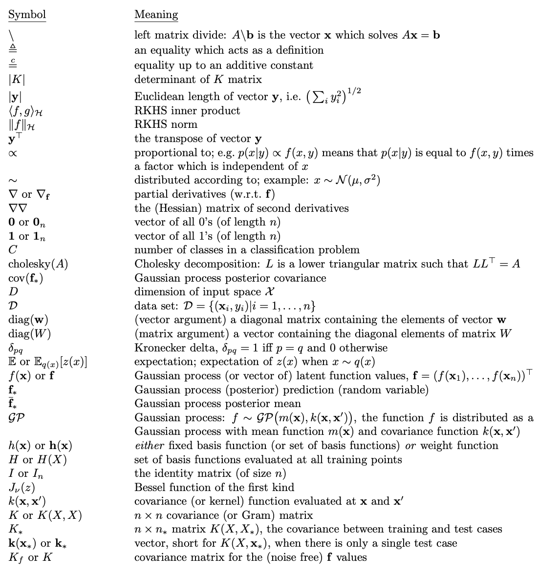
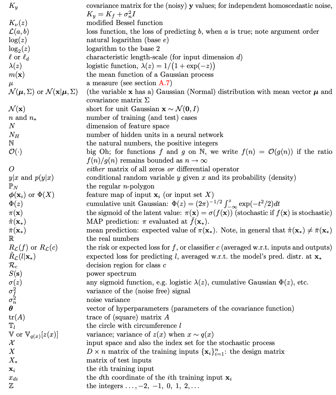
Notations

Gaussian Identities

The multivariate Gaussian distribution has a joint probability density (Bayesian):

\[p(\mathbf{x} | \mathbf{m}, \Sigma) = (2\pi)^{-\frac{D}{2}} |\Sigma|^{-\frac{1}{2}} e^{-\frac{1}{2} (\mathbf{x} - \mathbf{m})^T \Sigma^{-1} (\mathbf{x} - \mathbf{m})}\]

Where \(\mathbf{m}\) is the mean vector of length \(D\) and \(\Sigma\) is the symmetric \(D \times D\), positive definite covariance matrix. As a shorthand, we write \(\mathbf{x} \sim N(\mathbf{m}, \Sigma)\)

Let \(\mathbf{x}, \mathbf{y}\) be jointly Gaussian random vectors:

$$$$

Regression

A Function Space View

Definition 2.1: Gaussian Process

A Gaussian Process is a collection of random variables, any finite number of which have joint Gaussian distribution.

A Gaussian process is completely specified by its mean function and covariance function. We define mean function \(m(\mathbf{x})\) and the covariance function \(k(\mathbf{x}, \mathbf{x}^\prime)\) of a real process \(f(\mathbf{x})\) as:

\[m(\mathbf{x}) = E[f(\mathbf{x})] \quad \quad k(\mathbf{x}, \mathbf{x}^\prime) = E[(f(\mathbf{x}) - m(\mathbf{x}))(f(\mathbf{x}^\prime) - m(\mathbf{x}^\prime))]\]

and given \(N\) examples, we write the Gaussian process \(f := (f(\mathbf{x}_1) , ...., f(\mathbf{x}_N))\) as:

\[f(\mathbf{x}) \sim GP(m(\mathbf{x}), k(\mathbf{x}, \mathbf{x}^\prime))\]

where the random variables represent the value of the function \(f\) at location \(\mathbf{x}\). Often Gaussian process are defined over time, where the index set of the random variables is time. This is not the case in our use of GPs, here the index set \(\mathbb{X}\) is the set of possible inputs. In our case, we identify the random variables s.t \(f_i := f(\mathbf{x}_i)\) corresponding to training example \((\mathbf{x}_i, y_i)\).