VAE

Variational Autoencoders

Generative modeling is a broad area of machine learning which deals with models of distributions \(P(X)\), defined over datapoints \(X\) in some potentially high-dimensional space \(\mathbf{X}\). For example, images are popular kind of data for which we might create generative models, the job of the generative model is to capture the dependencies between pixels and model the joint distribution between them. One straight forward kind of generative model is simply to compute the probability measure \(P(X)\) numerically, given a \(X\), we can tell the probability that \(X\) is a real image from the distribution. But we often care about producing more examples that are like those already in a database, that is, we can formalize the setup by saying that:

we get examples \(X\) distributed according ot some unknown distribution \(P_{gt} (X)\), and our goal is to learn a model \(P\) which we can sample from , such that \(P\) is as similar as possible to \(P_{gt}\).

Formally, say we have a vector of latent variables \(\mathbf{z}\) that have values in some high-dimensional space \(\mathbf{Z}\) which we can easily sample according to some probability density function \(P(\mathbf{z})\) defined over \(\mathbf{Z}\). Then, say we have a family of deterministic functions \(f(\mathbf{z}; \theta)\), parameterized by a vector \(\theta\) values in some space \(\Theta\), where:

\[f(\mathbf{z}; \theta);\quad f: \mathbf{Z} \times \Theta \rightarrow \mathbf{X}\]

\(f\) is deterministic, but if \(\mathbf{z}\) is random, then \(f(\mathbf{z}; \theta) := f(\cdot; \theta) \circ \mathbf{z}\) is a random variable with values in \(\mathbf{X}\). We wish to optimize \(\theta\) s.t we can sample \(\mathbf{z}\) from \(P(\mathbf{z})\) and with high probability \(f(\mathbf{z}; \theta)\) will be like the \(X\)s' in our datasets. That is, we aim to maximize the probability of each \(X\) in the training set under the entire generative process (Maximize the likelihood):

\[P(X) = \int P(X| \mathbf{z}; \theta) P(\mathbf{z}) d\mathbf{z} \quad \quad (1)\]

The intuition behind this framework: If the model is likely to produce training examples, then it is likely to produce similar samples and unlikely to produce dissimilar ones.

In VAE, conditional density \(P(X | \mathbf{z};\theta)\) is often parameterized by Multivariate Gaussian (with parameterized mean function, we can approach \(X\) for some \(\mathbf{z}\), gradually making the training data more likely under the generative model.):

\[P(X | \mathbf{z}; \theta) = N(X | f(\mathbf{z}\; \theta), \sigma^2 I)\]

But it is not required to be Gaussian, if \(X\) is binary, \(P(X | \mathbf{z})\) might be a Bernoulli, the important property is simply that \(P(X | \mathbf{z})\) can be computed and is continuous in \(\theta\).

Setting up the Objective

How can we estimate equation 1 using sampling? In practice, for most \(\mathbf{z}\), \(P(X | \mathbf{z})\) will be nearly zero, so it contributes nothing to \(P(X)\). The key idea behind the VAE is to attempt to sample values \(\mathbf{z}\) that are likely to have produced \(X\), and compute \(P(X)\) from there. This means we need a new function \(Q(\mathbf{z} | X)\) which can take a value of \(X\) and give us a distribution over \(\mathbf{z}\) values that are likely to produce \(X\). Thus, computing \(E_{ \mathbf{z} \sim Q} [P(X | \mathbf{z})]\) is much easier than \(E_{ \mathbf{z} \sim P( \mathbf{z})}[P(X | \mathbf{z})]\).

The KL divergence between \(Q(\mathbf{z} | X)\) and \(P(\mathbf{z} | X)\) is:

\[D[Q(\mathbf{z} | X) || P(\mathbf{z} | X)] = E_{z \sim Q} [\log Q(\mathbf{z} | X) - \log P(\mathbf{z} | X)]\]

Use bayes rule:

\[\log P(X) - D[Q(\mathbf{z} | X) || P(\mathbf{z} | X)] = E_{z \sim Q} [\log P(X | \mathbf{z})] - D[Q(\mathbf{z} | X) || P(\mathbf{z})]\]

Starting from left-hand side, we are maximizing the log evidence while simultaneously minimizing the distribution regularization term. The right-hand side (ELBO) is similar to auto-encoder, where we map \(X \rightarrow \mathbf{z}\) using \(Q\), then decode back to \(X\) using \(P\).

The right-hand side can be optimized using gradient decent.

Optimize the Objective

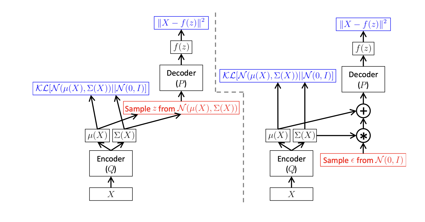
How can we optimize the right-hand side (ELBO) ? we first need to be a bit more specific about the form that \(Q(\mathbf{z} | X)\) will take. The usual choice is to say that \(Q(\mathbf{z} | X) = N(\mathbf{z} | \mu(X), \Sigma(X))\), in practice, \(\mu, \Sigma\) are parametrized using NN.