Base on Fourier Analysis: an Introduction by Elias M. Stein & Rami Shakarchi

Fourier Analysis (1)

Basic Properties of Fourier Series

Key Takeaway

Preliminary

Useful Identities

• \(e^{ix} = \cos(x) + i\sin(x)\)
• \(\cos(x) = \frac{e^{ix} + e^{-ix}}{2}\)
• \(\sin(x) = \frac{e^{ix} - e^{-ix}}{2i}\)

Complex Trigonometric Polynomial

Any function \(T\) of the form:

\[T(x) = a_0 + \sum^N_{n=1}a_n \cos(nx) + \sum^N_{n=1} b_n \sin(nx)\]

with \(a_n, b_n \in \mathbb{C}, 0 \leq n \leq \mathbb{N}, x \in \mathbb{R}\) is called a Complex Trigonometric Polynomial, it can also be written as:

\[T(x) = \sum^N_{n=-N} c_n e^{inx}\]

Everywhere continuous functions

These are the complex-valued functions \(f\) which are continuous at every point of the segment \([0, L]\). Continuous functions on the circle satisfy the additional condition \(f(0) = f(L)\). (starting point = end point)

Piecewise continuous functions

These are bounded functions on \([0, L]\) which have only finitely many discontinuities.

Riemann integrable functions

Refer to Theorem 3.34 of MIRA(2). We say that a complex-valued function is integrable (Riemann) if its real and imaginary parts are integrable. The sum and product of two integrable functions are integrable.

Functions on the circle

A point on the unit circle takes the form \(e^{i\theta}\) (mapping from real number to number on a unit circle), where \(\theta\) is a real number unique up to integer multiples of \(2\pi\). If \(F\) is a function on the circle, then we may define for every \(\theta \in \mathbb{R}\):

\[f(\theta) = F(e^{i\theta})\]

\[f(\theta + 2\pi) = f(\theta), \quad \forall \theta \in \mathbb{R}\]

In conclusion, functions on \(\mathbb{R}\) that \(2\pi-\)periodic, and functions on an interval of length \(2\pi\) that take on the same value at its end-points are two equivalent descriptions of the same mathematical objects, namely, functions on the circle.

Main Definitions

• All functions are assumed to be integrable (Riemann).

Def 1.1.1: Fourier Coefficient and Fourier Series of a Function

If \(f\) is an integrable function given on an interval \([a, b]\) of length \(L = b - a\), then the \(n\)th Fourier coefficient of \(f\) is defined by:

\[\hat{f}(n) = \frac{1}{L} \int^b_a f(x) e^{-2\pi inx / L} dx, \quad n \in \mathbb{Z}\]

If f is period, then the \(\hat{f}(n)\) is independent of the choice of interval (same for all intervals).

The Fourier series of \(f\) is given by :

\[\sum^{\infty}_{n=-\infty} \hat{f}(n) e^{2\pi inx / L}\]

Def 1.1.2: Dirichlet Kernel

The trigonometric polynomial defined for \(x \in [-\pi, \pi]\) by:

\[D_N(x) = \sum^N_{n=-N} e^{inx} = \frac{\sin((N + \frac{1}{2})x)}{\sin(\frac{x}{2})}\]

is called the \(Nth\) Dirichlet kernel. The Fourier coefficients \(a_n\) have the property that \(a_n = 1\) if \(|n| \leq N\) and \(a_n = 0\) otherwise.

Def 1.1.3: Poisson Kernel

The function \(P_r(\theta)\), is called the Poisson kernel, is defined for \(\theta \in [-\pi, \pi]\) and \(0 \leq r < 1\) by the absolutely and uniformly convergent series:

\[P_r(\theta) = \sum^\infty_{n=-\infty} r^{|n|}e^{in\theta}\]

Uniqueness of Fourier Series

Theorem 2.1 Continuous points have value zero when all Fourier coefficients are zeros

Suppose that \(f\) is an integrable function on the circle with \(\hat{f}(n) = 0\) for all \(n \in \mathbb{Z}\). Then \(f(\theta_0) = 0\) whenever \(f\) is continuous at the point \(\theta_0\).

Corollary 2.2:

If \(f\) is continuous on the circle and \(\hat{f}(n) = 0\) for all \(n \in \mathbb{Z}\), then \(f = 0\).

Theorem 2.3: If series of Fourier Coefficients converges absolutely, then Fourier Series converges to \(f\)

Suppose that \(f\) is a continuous function on the circle and that the Fourier coefficients of \(f\) is absolutely convergent, \(\sum^\infty_{n = -\infty} |\hat{f}(n)| < \infty\). Then, the Fourier series converges uniformly to \(f\), that is:

\[\lim_{N\rightarrow \infty} S_N (f) (\theta) = f(\theta)\]

uniformly in \(\theta\).

What conditions on f would guarantee the absolute convergence of its Fourier series? As it turns out, the smoothness of f is directly related to the decay of the Fourier coefficients, and in general, the smoother the function, the faster this decay. As a result, we can expect that relatively smooth functions equal their Fourier series.

\(C^k\)

We say that \(f\) belongs to the class \(C^k\) if \(f\) is \(k\) times continuously differentiable. This is a way to describe the smoothness of a function.

Convolution

Given two \(2\pi\)-periodic integrable functions \(f\) and \(g\) on \(\mathbb{R}\), we define their convolution \(f * g\) on \([-\pi, \pi]\) by:

\[(f * g) (x) = \frac{1}{2\pi} \int^{\pi}_{-\pi} f(y) g(x - y) dy\]

For \(2\pi\)-periodic functions, these two forms are equivalent:

\[(f * g) (x) = \frac{1}{2\pi} \int^{\pi}_{-\pi} f(x - y) g(y) dy\]

Loosely speaking, convolutions correspond to "weighted averages", if \(g = 1\), then \(f * g (x) = \frac{1}{2\pi} \int^\pi_{-\pi} f(y) dy\) is a constant that represents the average value of \(f\) on the circle.

Partial Sums of Fourier Series of \(2\pi\) periodic function as Convolution

Given a \(2\pi\)-periodic integrable function \(f\), the Fourier Series of \(f\) can be expressed as:

\[S_N(f) (x) = \frac{1}{2\pi} \int^\pi_{-\pi} f(y) (\sum^N_{n=-N} e^{in(x - y)}) dy = (f * D_N) (x)\]

where \(D_N(x)\) is the Dirichlet kernel.

Proposition 3.1:

Suppose that \(f, g, h\) are \(2\pi\) periodic integrable functions. Then:

1. \(f * (g + h) = (f * g) + (f * h)\) (linearity)
2. \((cf) * g = c(f * g) = f * (cg), \;\;\forall c \in \mathbb{C}\) (commutativity)
3. \(f * g = g * f\)
4. \((f * g) * h = f * (g * h)\) (associativity)
5. \((f * g)\) is continuous. (The convolution of two integrable function is more regular.)
6. \(\widehat{f * g} (n) = \hat{f}(n) \hat{g}(n)\)

Good Kernels

A family of kernels \(\{K_n(x)\}^\infty_{n=1}\) on the circle is said to be a family of good kernels if it satisfies the following properties:

1. For all \(n \geq 1\), (The average value on the circle is 1) \[\frac{1}{2\pi} \int^{\pi}_{-\pi} K_n(x) dx = 1\]
2. There exists \(M > 0\) s.t for all \(n \geq 1\) (The integral is bounded), \[\int^\pi_{-\pi} |K_n(x)|dx \leq M\]
3. For every \(\delta > 0\), \[\int_{\delta \leq |x|\leq \pi} |K_n(x)|dx \rightarrow 0, \;\; \text{as} \; n \rightarrow \infty\]

Theorem 4.1: Approximation to Identity

Let \(\{K_n\}^\infty_{n=1}\) be a family of good kernels, and \(f\) an integrable function on the circle. Then,

\[\lim_{n \rightarrow \infty} (f * K_n) (x) = f(x)\]

whenever \(f\) is continuous at \(x\). if \(f\) is continuous everywhere, then the above limit is uniform. Because of this result, the family \(\{K_n\}\) is sometimes referred to as an approximation to the identity.

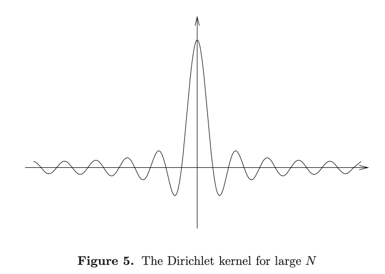
The Dirichlet kernel satisfies condition 1 of the good kernel but does not satisfy condition 2:

\[D_N(x) \geq c\log N\]

Convergence of Fourier Series

Mean-square Convergence on Circle

If \(f\) is integrable on the circle, then:

\[\frac{1}{2\pi} \int^{2\pi}_{0} |f(\theta) - S_N(f)(\theta)|^2 d\theta \rightarrow 0, \;\; n \rightarrow \infty\]

or

\[\lim_{N \rightarrow \infty} E[(f - S_N(f))^2]\]

Fourier Transform

The theory of Fourier series applies to functions on the circle. In this section we develop an analogous theory for functions on the entire real line which are non-periodic. Roughly speaking, the Fourier Transform is a continuous version of the Fourier coefficients. The Fourier inversion formula is a continuous version of the Fourier series.

Elementary Theory of The Fourier Transform

Given the notion of the integral of a function on a closed and bounded interval, the most natural extension of this definition to continuous functions over \(\mathbb{R}\) is:

\[\int^\infty_{-\infty} f(x)dx = \lim_{N \rightarrow \infty} \int^N_{-N} f(x) dx\]

The limit may not exists (e.g., $f(x ) = 1 $), but if we let \(f\) decay enough as \(|x| \rightarrow \infty\), it will exist.

A function \(f\) defined on \(\mathbb{R}\) is said to be of moderate decreasing if \(f\) is continuous and there exists a constant \(A > 0\) so that:

\[|f(x)| \leq \frac{A}{1 + x^{1 + \epsilon}}, \;\; \forall x \in \mathbb{R}\]

The function of moderate decreasing is bounded (by \(A\)) and decays at infinity at least as fast as \(1 / x^2\), we denote the set of all moderate decreasing functions as \(M(\mathbb{R})\), we can show that it is a vector space over \(\mathbb{C}\).

If the function is moderate decreasing, then we can be sure that the limit exists and the sequence of integral converges.

Theorem 5.1: Properties of Improper Integral

The integral of a function of moderate decrease (i.e., \(f \in M(\mathbb{R})\)) satisfies the following properties:

1. Linearity: If \(f, g \in M(\mathbb{R})\) and \(a, b \in \mathbb{C}\), then: \[\int^\infty_{-\infty} (af(x) + bg(x))dx = a\int^\infty_{-\infty} f(x)dx + b\int^\infty_{-\infty} g(x)dx\]
2. Translation Invariance: For every \(h \in \mathbb{R}\) we have: \[\int^\infty_{-\infty} f(x - h) dx = \int^\infty_{-\infty} f(x) dx\]
3. Scaling under dilations: If \(\delta > 0\), then: \[\delta \int^\infty_{-\infty} f(\delta x)dx = \int^\infty_{-\infty} f(x) dx\]
4. Continuity: If \(f \in M(\mathbb{R})\), then: \[\int^\infty_{-\infty} |f(x - h) - f(x)| dx \rightarrow 0, \;\; \text{as } h \rightarrow 0\]

Definition of the Fourier transform

If \(f \in M(\mathbb{R})\), we define the Fourier transform for \(\xi \in \mathbb{R}\) by:

\[\hat{f}(\xi) = \int^{\infty}_{-\infty} f(x) e^{-2\pi \xi x i} dx\]

Notice that, \(\hat{f}\) is continuous and bounded, \(|e^{-2\pi \xi x i}| = 1\).

The Schwartz Space

The Schwartz space on \(\mathbb{R}\) consists of the set of all indefinitely differentiable functions \(f\) so that \(f\) and all its derivatives \(f^\prime, f^{\prime\prime}, ...., f^{l}, ...\) are rapidly decreasing, in the sense that:

\[\sup_{x \in \mathbb{R}} |x|^k |f^{l} (x)| < \infty, \;\; \forall k, l > 0\]

We denote this space by \(S = S(\mathbb{R})\):

• \(S\) is a vector space
• If \(f \in \mathbb{R}\), then \(f^{\prime} \in S(\mathbb{R})\) (closed under differentiation), \(x f(x) \in \mathbb{R}\) (closed under polynomial).
• \(f(x) = e^{-ax^2}, \; a > 0\) is an example of the elements in \(S\).

Fourier Transform on \(S\)

The Fourier Transform of a function \(f \in S(\mathbb{R})\), \(F(f) = \hat{f}: S(\mathbb{R}) \rightarrow S(\mathbb{R})\) is defined by:

\[\hat{f}(\xi) = \int^{\infty}_{-\infty} f(x) e^{-2\pi i x \xi} dx\]

Some properties hold for Fourier Transform of a function \(f \in S(\mathbb{R})\), we denote the fourier transform of \(f\) by:

\[f(x) \rightarrow \hat{f}(\xi)\]

• \(f(x + h) \rightarrow \hat{f}(\xi) e^{2\pi i h \xi}, \;\; \forall h \in \mathbb{R}\)
• \(f(x) e^{-2\pi i x h} \rightarrow \hat{f} (\xi + h), \;\; \forall h \in \mathbb{R}\)
• \(f(\delta x) \rightarrow \delta^{-1} \hat{f}(\delta^{-1}\xi), \;\; \forall h \in \mathbb{R}\)
• \(f^{\prime}(x) \rightarrow 2\pi i \xi \hat{f}(\xi)\)
• \(-2\pi i x f(x) \rightarrow \frac{d}{d\xi} \hat{f}(\xi)\)
• \(\hat{\bar{f}} (x) = \overline{\hat{f}(-\xi)}\)

Theorem 5.2

If \(f \in S(\mathbb{R})\), then \(\hat{f} \in S(\mathbb{R})\).

Gaussians (\(e^{-ax^2}\)) are Good Kernels

\[\int^{\infty}_{-\infty} e^{-\pi x^2} dx = 1\]

Theorem 5.4 The Fourier Transform of \(e^{-\pi x^2}\) is itself

If \(f(x) = e^{-\pi x^2}\), then \(\hat{f}(\xi) = f(\xi)\)

Theorem 5.5

If \(\delta > 0\) and \(K_{\delta} (x) = \delta^{-\frac{1}{2}} e^{\frac{-\pi x^2}{\delta}}\), then \(\hat{K}_{\delta}(\xi) = e^{-\pi \delta \xi^2}\)

Proof of Theorem 5.5

\[K_{\delta} (x) = \delta^{-\frac{1}{2}} e^{\frac{-\pi x^2}{\delta}} = \delta^{-\frac{1}{2}}f(\delta^{-\frac{1}{2}} x)\]

where \(f(\delta^{-\frac{1}{2}} x) = e^{-\pi \frac{x^2}{\delta}}\)

Then:

\[\hat{K}_\delta(x) = \delta^{\frac{1}{2}}\hat{f}^\prime(\delta^{\frac{1}{2}}\xi) = e^{-\pi \delta \xi^2}\]

Theorem 5.6: \(\{K_{\delta}\}_{\delta > 0}\) is a Family of Good Kernels

\(\{K_{\delta} (x)\}_{\delta \in \mathbb{R^+}} = \delta^{-\frac{1}{2}} e^{\frac{-\pi x^2}{\delta}}\) is a family of good kernels as \(\delta \rightarrow 0\).

Convolution on \(\mathbb{R}\)

If \(f, g \in S(\mathbb{R})\), then the convolution is defined by:

\[(f * g) (x) = \int^{\infty}_{-\infty} f(x - t) g(t) dt\]

for a fixed value \(x\), the function \(f(x - t) g(t)\) is rapid decrease in \(t\).

Theorem 5.7

If \(f \in S(\mathbb{R})\), then

\[(f * K_{\delta}) (x) \rightarrow f(x), \;\; \text{uniformly in $x$ as $\delta \rightarrow 0$}\]

The Fourier Inversion

Theorem 5.8: The Multiplication Formula

If \(f, g \in S(\mathbb{R})\), then

\[\int^{\infty}_{-\infty} f(x)\hat{g}(x) dx = \int^{\infty}_{-\infty} \hat{f}(y) g(y) dy\]

Theorem 5.9: Fourier Inversion

If \(f \in S(\mathbb{R})\), we define the inversion \(F^* (\hat{f}) : S(\mathbb{R}) \rightarrow S(\mathbb{R})\) by

\[F^* (\hat{f}) (x)= \int^{\infty}_{-\infty} \hat{f}(\xi) e^{2\pi i x\xi} dx\]

Then:

\[F^*(\hat{f}) (x) = f(x)\]

Theorem 5.10: Fourier Transform is a Bijective Mapping on the Schwartz Space

The Fourier transform is a bijective mapping on the Schwartz space.

Theorem 5.11: Convolutions of Schwartz Functions

If \(f, g \in S(\mathbb{R})\), then:

1. \(f * g \in S(\mathbb{R})\)
2. \(f * g = g * f\)
3. \((\widehat{f * g}) (\xi) = \hat{f}(\xi)\hat{g}(\xi)\)

Inner Product in Schwartz Space

The Schwartz space can be equipped with a Hermitian inner product:

\[<f, g> = \int^{\infty}_{-\infty} f(x) \bar{g}(x) dx\]

whose associated norm is:

\[\|f\| = \sqrt{\int^{\infty}_{-\infty} |f(x)|^2 dx}\]

Theorem 5.12: Plancherel, The Norm of Fourier Transform Preserves

If \(f \in S(\mathbb{R})\) then \(\|\hat{f}\| = \|f\|\)

Extension to Functions of Moderate Decrease

All properties hold for \(f \in M(\mathbb{R})\)

Monomial \(x^\alpha\)

Given a \(d\)-tuple \(\alpha = (\alpha_1, ...., \alpha_d)\) of non-negative integers (multi-index), the monomial \(x^\alpha\) is defined by:

\[x^\alpha = x_1^{\alpha_1} x_2^{\alpha_2} ... x_d^{\alpha_d}\]

Rotation in \(\mathbb{R}^d\)

A rotation in \(\mathbb{R}^d\) is a linear transformation \(R: \mathbb{R}^d \rightarrow \mathbb{R}^d\) which preserves the inner product. In the other words,

• \(R(ax + by) = aR(x) + bR(y) \;\; \forall x, y \in \mathbb{R}^d, \; a, b \in \mathbb{R}\)
• \(R(x) \cdot R(y) = x \cdot y, \;\; \forall x, y \in \mathbb{R}^d\)

If \(\det{(R)} = 1\), \(R\) is a proper rotation, otherwise, we say that \(R\) is an improper rotation.

Rapid Decreasing of Complex Function on \(\mathbb{R}^d\)

A continuous complex-valued function \(f\) on \(\mathbb{R}^d\) is said to be rapidly decreasing if for every multi-index \(\alpha\) the function \(|x^\alpha f(x)|\) is bounded. Equivalently, a continuous function is of rapid decrease if:

\[\sup_{x \in \mathbb{R}^d} |x|^k |f(x)| < \infty, \quad\quad \forall k = 0, 1, 2, ...\]

Given a function of rapid decrease, we define:

\[\int_{\mathbb{R}^d} f(x) dx = \lim_{N \rightarrow \infty} \int_{Q_N} f(x) dx\]

Where \(Q_N\) denotes the closed cube centered at the origin, with sides of length \(N\) parallel to the coordinate axis, that is,

\[Q_N = \{x \in \mathbb{R}^d: |x_i| \leq \frac{N}{2} \quad \quad i = 1, ..., d\}\]

Actually, the limit exists if we can show that \(f\) is continuous and

\[\sup_{x \in \mathbb{R}^d} |x|^{d + \epsilon} |f(x)| < \infty, \quad \text{for some $\epsilon > 0$}\]

If the function \(f\) satisfies the condition with \(\epsilon = 1\), we say that the function is moderate decrease on \(\mathbb{R}^d\).

Properties of Moderate Decreasing Functions

If \(f\) is of moderate decrease, then:

1. Translation Invariant:

\[\int_{\mathbb{R}^d} f(x + h) dx = \int_{\mathbb{R}^d} f(x) dx \quad \forall h \in \mathbb{R}^d\]

2. Scaling Invariant:

\[\delta^d \int_{\mathbb{R}^d} f(\delta x) dx = \int_{\mathbb{R}^d} f(x) dx \quad \forall \delta > 0\]

3. Rotation Invariant:

\[\int_{\mathbb{R}^d} f(R(x)) dx = \int_{\mathbb{R}^d} f(x) \quad \text{$\forall$ rotation $R$}\]

Schwartz Space in \(\mathbb{R}^d\)

The Schwartz space \(S(\mathbb{R}^d)\) consists of all indefinitely differentiable functions \(f\) on \(\mathbb{R}^d\) such that

\[\sup_{x \in \mathbb{R}^d} |x^\alpha (\frac{\partial }{\partial x})^\beta f(x)| < \infty\]

for every multi-index \(\alpha, \beta\). In other words, \(f\) and all its derivative are required to be rapidly decreasing.

Fourier Transform on \(\mathbb{R}^d\)

The Fourier transform of a Schwartz function \(f\) is defined by:

\[\hat{f}(\xi) = \int_{\mathbb{R}^d} f(x) e^{-2\pi ix \cdot \xi} dx \quad \quad \text{for } \xi \in \mathbb{R}^d\]

This resembles with the formula in one-dimension, except we have dot product between \(\xi\) and \(x\) now.

Properties of Fourier Transform in \(\mathbb{R}^d\)

Let \(f \in \mathbb{R}^d\)

1. \(f(x + h) \rightarrow \hat{f}(\xi) e^{2\pi i \xi \cdot h}, \quad h \in \mathbb{R}^d\)
2. \(f(x) e^{-2\pi i x h} \rightarrow \hat{f} (\xi + h), \quad h \in \mathbb{R}^d\)
3. \(f(\delta x) \rightarrow \delta^{-d} \hat{f}(\delta^{-1} \xi), \quad \delta > 0\)
4. \((\frac{\partial }{\partial x})^\alpha f(x) \rightarrow (2\pi i \xi)^\alpha \hat{f}(\xi)\)
5. \((-2\pi i x)^\alpha f(x) \rightarrow (\frac{\partial }{\partial x})^\alpha \hat{f}(\xi)\)
6. \(f(Rx) \rightarrow \hat{f}(R\xi), \quad R \text{ is a rotation}\)

Fourier Inversion in \(\mathbb{R}^d\)

Suppose \(f \in S(\mathbb{R}^d)\). Then:

\[f(x) = \int_{\mathbb{R}^d} \hat{f}(\xi) e^{2\pi i x \cdot \xi} d\xi\]

Moreover

\[\int_{\mathbb{R}^d} |\hat{f}(x)|^2 d\xi = \int_{\mathbb{R}^d} |f(x)|^2 dx\]

Finite Fourier Analysis

Binary Relation

A binary (two element) relation from a set \(X\) to a set \(Y\) is a subset of the cartesian product \(X \times Y\), where \(X\) is called domain and \(Y\) is called the codomain. If an ordered pair \((x, y)\) is in a relation \(R\), then the relation holds true for \((x, y)\). A binary relation on a set \(S\) is a subset of the cartesian product \(S \times S\). We use \(xRy\) or \(x \sim y\) to denote the ordered pair \((x, y)\) is in relation \(R\).

If \(S = \{1, 2, 3\}\) then \(x < y\) on \(S\) is a relation \(R = \{(1, 2), (2, 3)\}\).

Equivalence Class and Equivalence Relation

A relation \(\sim\) on a set \(S\) is an equivalence relation if:

1. (Reflexivity) \(s \sim s \; \forall s \in S\).
2. (Symmetry) \(\forall \; s, t \in S\), if \(s \sim t\), then \(t \sim s\).
3. (Transitivity) \(\forall \; s, t, u \in S\), if \(s \sim t\) and \(t \sim u\), then \(s \sim u\).

An equivalence relation is meant to capture the idea of things "being the same" for the purposes of a given discussion.

Congruent mod \(n\)

Let \(n \in \mathbb{Z}^+\) be a positive integer, integers \(x, y\) are congruent mod \(n\) if \(x - y\) is divisible by \(n\). Congruent mod \(n\) is an equivalence relation on \(\mathbb{Z}\).

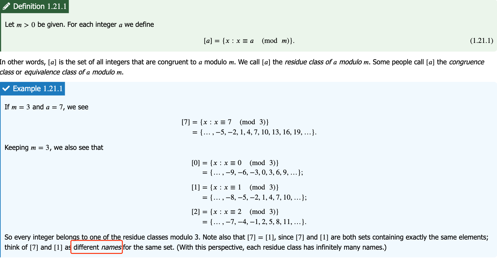
Residue Class

A residue class \(R(r)\) is a complete set of integers that are congruent modulo \(n\) with reminder \(r\) (ie. \(a = kn + r \implies a \in R(r), \; k \in \mathbb{Z}, n \in \mathbb{Z}^+, 0 \leq r \in \mathbb{Z} leq n - 1\)). In module \(n\), there are exactly \(n\) different residue classes.

Binary Operation

A binary operation on a set \(S\) is a mapping of the elements of the Cartesian product \(S \times S\) to \(S\):

\[f: S \times S \rightarrow S\]

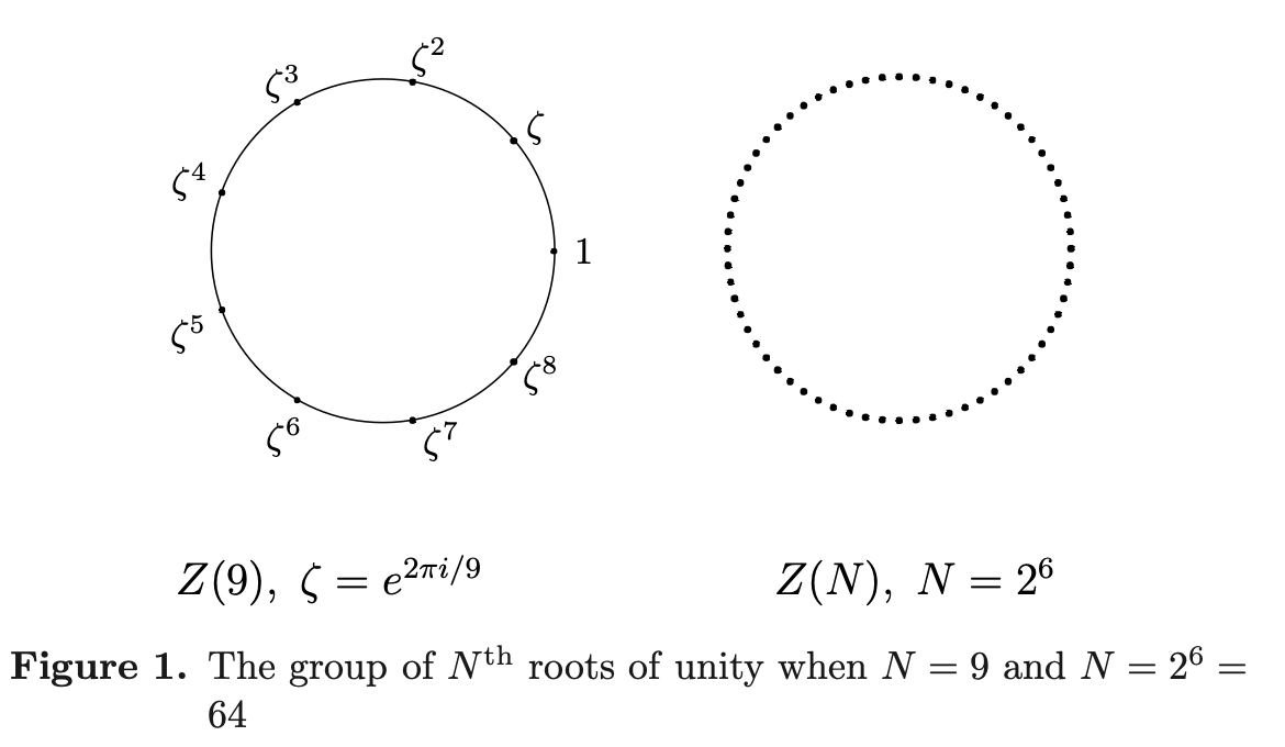
The group \(Z(N)\)

Let \(N\) be a positive integer. A complex number \(z\) is an \(N^{th}\) root of unity if \(z^N = 1\). The set of \(N^{th}\) roots of unity is precisely:

\[\{1, e^{2\pi i / N}, e^{2\pi i 2 / N}, ...., e^{2\pi i (N - 1) / N}\}\]

This is uniform partition of the circle.

The set has the following properties:

1. If \(z, w \in Z(N)\), then \(zw \in Z(N)\) and \(zw = wz\)
2. \(1 \in Z(N)\)
3. If \(z \in Z(N)\), then \(z^{-1} = \frac{1}{z} \in Z(N)\) and \(z z^{-1} = 1\)

The group \(Z(N)\) is equivalent to the group of integers modulo \(N\) which contains integers $0 n + m $

Let \(V, W\) denote the vector spaces of complexed-valued functions on the group of integers modulo \(N\) and the \(N\)th roots of unity. Then, the identification given above carries over to \(V, W\) as follows:

\[F(k) \longleftrightarrow f(e^{2\pi i k/N})\]

Where \(F\) is a function on \(V\) and \(f\) is a function on the \(W\). These spaces can be represented as \(\mathbb{Z}(N)\), because they are equivalent.

Orthogonal Bases in \(\mathbb{Z}(N)\)

The family \(\{e_{0}, ...., e_{N-1}\}\) is an orthogonal basis of vector space \(\mathbb{Z}(N)\) equipped with inner product

\[<F, G> = \sum^{N-1}_{k=0} F(k) \overline{G(k)}\]

and corresponding norm:

\[\|F\| = \sqrt{\sum^{N-1}_{k=0} F(k) \overline{F(k)}} = \sqrt{\sum^{N-1}_{k=0} |F(k)|^2}\]

where:

\[e_{l} (k) = e^{2\pi i lk/n}\]

and: \[ <e_m, e_l> = \begin{cases} N & \quad \text{If $m = l$} \\ 0 & \quad \text{If $m \neq l$} \end{cases} \]

Since all \(e_l\) has norm \(\sqrt{N}\), if we normalize it by \(\frac{1}{\sqrt{N}}\), we will have an orthnormal basis \(\{e^*_0, ...., e^*_{N-1}\}\):

\[e^*_l = \frac{1}{\sqrt{N}} e_l\]

Thus, for any \(F \in V\), we have:

\[F = \sum^{N-1}_{n=0} <F, e^*_n> e^*_n\]

and

\[\|F\|^2 = \sum^{N-1}_{n=0} |<F, e^*_n>|^2\]

Fourier Coefficient in \(\mathbb{Z}(N)\)

Define \(n\)th Fourier Coefficient of \(F\) by:

\[a_n = \frac{1}{N} <F, e_n> = \frac{1}{N} \sum^{N-1}_{k=0} F(k) e^{-2\pi i k n /N}\]

At the same time:

\[a_n = \frac{1}{\sqrt{N}} <F, e^*_n>\]

The function \(\hat{F}(n) = a_n\) is the Fourier transform of \(F\) on \(\mathbb{Z}(N)\).

Inversion Formula

If \(F\) is a function on \(\mathbb{Z}(N)\), then:

\[F(k) = \sum^{N-1}_{n=0} <F, e^*_n> e^*_n = \sum^{N-1}_{n=0} a_n e^{2\pi i n k / N} = \sum^{N-1}_{n=0} \hat{F}(n) e^{2\pi i n k / N}\]

It is possible to recover the Fourier inversion on the circle for sufficiently smooth function by letting \(N \rightarrow \infty\) in the finite model \(\mathbb{Z}(N)\).

Discrete Fourier Transform

When a signal is discrete and periodic, we don't need the continuous Fourier Transform. Instead, we use discrete Fourier Transform or DFT. Suppose our signal is \(a_n\) for \(n = 0, ...., N-1\) and \(a_n = a_{n + jN}\) ofr all \(n, j\). The DFT of \(a\), also known as the spectrum of \(a\) is \(F(n)\):

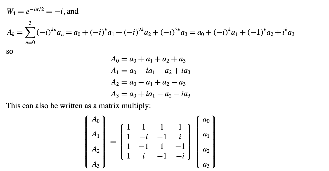
\[\hat{F}(k) = A_k = <a, e_k> = \sum^{N-1}_{n=0} e^{-2\pi i kn / N} a_n\]

The sequence \(a_n\) is the inverse discrete Fourier Transform of the sequence \(A_k\):

\[a_n = \frac{1}{N}\sum^{N-1}_{k=0} <a, e_k> e_k = \frac{1}{N} \sum^{N-1}_{k=0} \hat{F}(k) e^{2\pi i n k / N}\]

Two Point DFT

\(N = 2\), \(e_1 (k) = e^{-i \pi} = -1, \forall k\), then:

\[A_k = (-1)^{kn} a_n = a_0 - (-1)^k a_1\]

Thus,

\[A_0 = a_0 + a_1\] \[A_1 = a_0 - a_1\]

\[ A = \begin{bmatrix} 1 & 1\\ 1 & -1 \end{bmatrix} \begin{bmatrix} a_0 \\ a_1 \end{bmatrix} \]

Four Point DFT

REF

1. https://sites.millersville.edu/bikenaga/math-proof/relations/relations.html
2. https://math.libretexts.org/Bookshelves/Combinatorics_and_Discrete_Mathematics/Elementary_Number_Theory_(Barrus_and_Clark)/01%3A_Chapters/1.21%3A_Residue_Classes_and_the_Integers_Modelo_m
3. Fourier Transforms and the ast Fourier Transform (FFT) Algorithm