Dropout: A Simple Way to Prevent Neural Networks from Overfitting

The key idea of drop out is to randomly drop units along with their connections from the neural network during training to prevent overfitting. It can be interpreted as a way of regularizing a NN by adding noise to its hidden units.

Introduction

With unlimited computation, the best way to "regularize" a fixed-sized model is to average the predictions of all possible settings of the parameters, weighting each setting by the posterior probability given the training data (\(P(\theta | X)\)). This approach is not feasible in real life especially when there is large computational cost for training neural networks and training data are limited.Dropout prevents overfitting and provides a way of approximately combining exponentially many neural network architectures effectively.

Dropout temporarily removes units from the network along with all their incoming and outgoing connections. The choice of which units to drop is random.

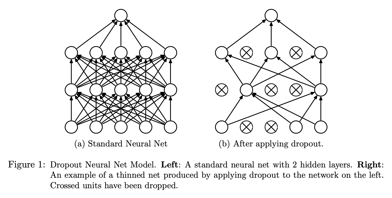
At training time, for a NN with \(n\) units, Dropout can be seen as training a collection of \(2^n\) (each unit can be retained or removed by dropout, so \(2^n\) different combinations) thinned networks (some units are dropped by dropout) with extensive weight sharing where each thinned network gets trained very rarely.

At test time, it is not feasible to explicitly average the predictions form exponentially many thinned models. However, we use a single NN without dropout by scaling-down the weights of this network. If an unit is retained with probability \(p\) during traning, the outgoing weights of that unit are multiplied by \(p\) at the test time. This ensures that the expected output is the same as the actual output at the test time (we use expected output at test time).

Policy Search Methods (Introduction)

So far, we have encountered methods for computing the optimal policy based on the computation of the value function. In this case, only value function was explicitly represented. There are also methods based on explicit representation of the policy and optimizing the performance of the agent by searching in the space of policies. These methods are called policy search methods.

Consider a stochastic policy \(\pi_\theta: X \rightarrow M(A)\) that maps state space to distribution defined over actions and parameterized by a \(\theta \in \Theta\). The set \(\Theta\) is the parameter space. The space of all parameterized policies can be described as:

\[\prod_\Theta = \{\pi_\theta: X \rightarrow M(A): \theta \in \Theta\}\]

This space depends on the mapping \(\pi_\theta\) and \(\Theta\)

One example how we can parameterize policy by softmax distribution. Given a function mapping \(f_{\theta}: X \times A \rightarrow \mathbb{R}\), the probability of choosing action \(a\) at state \(x\) is:

\[\pi_{\theta} (a | x) = \frac{exp(f_{\theta} (x, a))}{\sum_{a^{\prime}} exp(f_{\theta} (x, a^{\prime}))}\]

or a normal distribution defined by \(\mu_\theta (x), \Sigma_\theta(x)\):

\[\pi_{\theta} (\cdot | x) = N(\mu_\theta(x), \Sigma_{\theta} (x))\]

Importance Sampling

Ref

https://www.quora.com/Why-doesn-t-DQN-use-importance-sampling-Dont-we-always-use-this-method-to-correct-the-sampling-error-produced-by-the-off-policy https://danieltakeshi.github.io/2019/01/25/deep-learning-01/

Prioritized Experience Replay

Introduction

In simplest form, RL agents observe a stream of experience and discard incoming data immediately, after a single update. Two issues with this are:

1. Strongly correlated updates that break the i.i.d assumptions of most stochastic-gradient-based algorithms
2. The rapid forgetting of possibly rare experiences that would be useful later on (ie. some rare actions, rare states etc)

Experience replay addresses both of these issues. In general, it can reduce the amount of experience required to learn, and replace it with more computation and more memory.

However, RL gant can learn more effectively from some transitions than from others. Transitions may be more or less surprising, redundant, or task-relevant. Some transitions may not be immediately useful to the agent but might become so when the agent competence increases. Prioritized replay memory liberates agents from considering transitions uniformly. In particular, the authers propose to more frequently reply transitions with high expected learning progress, as measured by the magnitude of their TD error (on expectation, it is the BR). The bias will be corrected with importance sampling, loss of diversity will be alleviated with stochastic optimization.

Using a replay memory leads to design choices at two levels: which experiences to store, and which experiences to replay (and how to do so). This paper addresses only the latter: making the most effective use of the replay memory for learning.

题目库: [455, 605, 122, 435, 665, 763, 452, 167, 88, 142, 633, 680, 524, 69, 34, 81, 350, 154, 53, 35, 374, 367, 744, 287, 1170, 1337, 153, 33, 154, 278]

Greedy

455 Easy

局部最优则全局最优, 将小的饼干满足胃口最小的孩子以此类推

1
2
3
4
5
6
7
8
9
10
11
12
13
14
15
16
17
18
19
20
21
22
23

class Solution:
    
    def findContentChildren(self, g: List[int], s: List[int]) -> int:

        g.sort()
        s.sort()
        num_people = 0
        curr_g = 0

        for i, v in enumerate(s):

            if curr_g >= len(g):

                break
            
            if v >= g[curr_g]:
                num_people += 1
                curr_g += 1
        
        return num_people
        

Cheat Sheet

Permutation and Combination

Number of permutations for \(n\) people and \(k\) chairs:

\[nPk = \frac{n!}{(n - k)!}\]

\[nCk = \frac{nPk}{k!} = \frac{n!}{k! (n - k)!}\]

RL

\[Q^{\pi} (s, a) = E_s^{\prime} [r + \gamma E_{a^{\prime}}[Q(s^{\prime}, a^{s^{\prime}}) | s^{\prime}] | s, a, \pi]\]

\[V^{*} (s) = max_{a} Q^{*} (s, a)\]

\[Q^{*} (s, a) = max_{\pi} Q^{\pi} (s, a), \forall (s, a) \in S X A\]

\[V^{\pi} (s) = E_{a_t \sim pi(\cdot | s)}[R_t | s_t=s, \pi] = E_{a_t \sim pi(\cdot | s)}[E[R_t | s_t, a_t, \pi] | s_t=s] = E_{a_t \sim pi(\cdot | s)}[ Q^{\pi}(s, a_t)]\]

\[A^{\pi} (s, a) = Q^{\pi} (s, a) - V^{\pi} (s)\]

\[E_{a}[A^{\pi} (s, a) | s] = E_{a}[Q^{\pi} (s, a) | s] - V^{\pi} (s) = 0\]

\[E_{s^{\prime}}[R_t + \gamma V^{\pi}(s^{\prime}) - V^{\pi} (s)] = A^{\pi}(s, a)\]

ML

True Positive Rate (Sensitivity or Recall):

\[\frac{TP}{TP + FN}\]

Specificity:

\[\frac{TN}{TN + FP}\]

False Positive Rate (1 - specificity):

\[\frac{FP}{TN + FP}\]

Precision:

\[\frac{TP}{TP + FP}\]

Accuracy:

\[\frac{TP + TN}{TP + TN + FP + FN}\]

F-score:

\[2 * \frac{Precision * Recall}{Precision + Recall}\]

SARSA

SARSA (State Action State Reward State Action) is an on-policy TD algorithm that follows a PI-like procedure:

1. Estimate \(Q^{\pi_k}\) for a given policy \(\pi_k\)
2. Perform policy improvement to obtain a new policy \(\pi_{k+1}\)

Compare with usual Policy iteration, SARSA uses Generalized policy iteration to improve the policy before \(Q\) converges to \(Q^{\pi_k}\).

Temporal Difference Learning for Control: Q-Learning

We can use TD-like methods for the problem of control too. Consider any \(Q\). Let \(X^{\prime} \sim P(\cdot | X, A)\) and \(R \sim R(\cdot | X, A)\) and define:

\[Y = R + \gamma max_{a^{\prime} \in A} Q(X^{\prime}, a^{\prime})\]

We have:

\[E[Y | X=x, A=a] = r(x, a) + \gamma \int P(dx^{\prime} | x, a) max_{a^{\prime} \in A} Q(x^{\prime}, a^{\prime}) = T^{*} Q (x, a)\]

So, \(Y\) is an unbiased estimate of \(T^{*} Q (x, a)\). Let's define the empirical Bellman optimality operator \(\hat{T}^{*} Q (x, a)\):

\[T^{*} Q (x, a) = Y = R + \gamma max_{a^{\prime} \in A} Q(X^{\prime}, a^{\prime})\]

We can write the SA update rule for estimating \(Q^{*}\) as:

\[Q_{t+1} (X_t, A_t) \leftarrow Q_t(X_t, A_t) + \alpha_t (X_t, A_t) [R_t + \gamma max_{a^{\prime} \in A} Q_t (X^{\prime}_t, a^{\prime}) - Q_t(X_t, A_t)]\]

Learning From Stream of Data (Temporal Difference Learning Methods)

We can see that from MC algorithm, in order to update \(\hat{Q^{\pi}}_{k+1} (x, a)\), we need to calculate the entire \(\hat{G^{\pi}_{k}}\) which involves sum over product of rewards. If each episode is long or even continuous, the calculation of \(\hat{G^{\pi}_{k}}\) will be hard or impossible. In general, MC is agnostic to the MDP structure, if the problem is an MDP, it does not benefit from the recursive property of the value functions.

TD methods benefit from the structure of the MDP even if we do not know the environment dynamics \(P\) and \(R\).

TD for Policy Evaluation

We first focus on VI for PE: at each state \(x\), the procedure is:

\[V_{k+1} (x) = T^{\pi} V_{k} (x) = r^{\pi} (x) + \gamma \int P(dx^{\prime} | x, a) \pi(da | x) V_{k} (x^{\prime})\]

If we do not know \(r^{\pi}, P\), we cannot compute this. Suppose that we have n samples starting from state \(x\), \(A_i \sim \pi(\cdot | x), X^{\prime}_i \sim P(\cdot | x, A_i), R_i \sim R(\cdot | x, A_i)\), using these samples and \(V_{k}\), we compute:

\[Y_i = R_i + \gamma V_{k} (X_i^{\prime})\]

Now, notice that:

\[E[R_i | X=x] = r^{\pi} (x)\]

and

\[E[V_{k} (X^{\prime}_i) | X=x] = \int P(dx^{\prime} | x, a) \pi(da | x)V_{k} (x^{\prime})\]

so the r.v $Y_i (x) $ (emphasis starting from state \(x\) )satisfies:

\[E[Y_i | X=x] = E[R_i + \gamma V_{k} (X_i^{\prime}) | X=x] = E[R_i | X=x] + \gamma E[V_{k} (X_i^{\prime}) | X=x] = T^{\pi} V_{k} (x)\]

This implies that \(Y_i\) is an unbiased estimator of \(T^{\pi} V_{k}\) evaluated at \(x\). Thus, we can use a sample mean of \(Y_i\) starting from \(x\) to estimate \(T^{\pi} V_k (x)\), or we can use SA procedure.

\[T^{\pi}V^{t+1}_{k} (x) \leftarrow (1 - \alpha_t) T^{\pi}V^{t}_{k} (x) + \alpha Y_i\]

Learning From Stream of Data (Monte Carlo Methods)

MC Policy Evaluation

The Goal is to learn or estimate the value function \(V^{\pi}\) and \(Q^{\pi}\) of a policy.

Recall that:

\[V^{\pi}(x) = E[G^{\pi}_{t} | X_t=x]\]

This is the expected return starting from state \(x\). At the same time, obtain a sample from return \(G^{\pi}\) is easy: if the agent starts at state \(x\), and follows \(\pi\), we can draw one sample of r.v \(G^{\pi}\) by computing the cumulative sum of rewards collected during the episode starting from the state \(x\):

\[\hat{G^{\pi}_{t}} = \sum^{\infty}_{k=t} \gamma^{k-t} R_{k}\]

If we repeat this process from the same state, we get another draw of r.v \(G^{\pi}\), let us call these samples \(G^{\pi (1)} (x)\), \(G^{\pi (2)} (x)\), ...., \(G^{\pi (n)} (x)\). We can get an estimate \(\hat{V^{\pi}} (x)\) of \(V^{\pi} (x)\) by taking the average of the sample average:

\[\hat{V^{\pi}} (x) = \frac{1}{n} \sum^{n}_{i=1} \hat{G}^{\pi(i)} (x)\]