Multivariate Calculus (1)

Fundamental Theorem of Calculus

If \(f\) is continuous and \(F\) is indefinite integral of \(f\) (i.e \(F^{\prime} = f\) or \(\int f(x) dx = F(x) + c\), without bounds) on closed interval \([a, b]\), then:

1. \(\int^{b}_{a} f(x) dx = F(b) - F(a)\)
2. \(\frac{d}{dx}\int^{x}_{a} f(t)dt = F^{\prime}(x) - F^{\prime}(a) = F^{\prime} (x) = f(x)\)

Definition of Integral

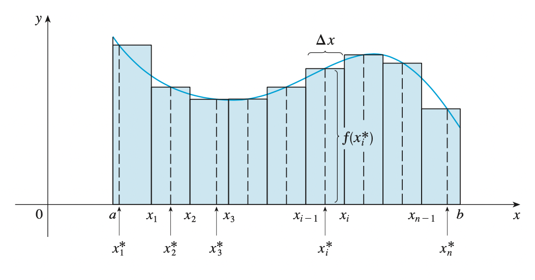
If \(f(x)\) is defined for \(a \leq x \leq b\), we start by dividing the interval \([a, b]\) into \(n\) sub-intervals \([x_{i - 1}, x_{i}]\) of equal width \(\Delta x = \frac{b - a}{n}\) and we choose sample points \(x^{*}_i\) in these subintervals. Then we form the Riemann sum:

\[\sum^{n}_{i=1} f(x^{*}_n) \Delta x\]

Then by taking the limit \(n \rightarrow \infty\), we have the definite integral of \(f\) from \(a\) to \(b\):

\[\int^{b}_{a} f(x) dx = \lim_{n \rightarrow \infty} \sum^{n}_{i=1} f(x^{*}_n) \Delta x\]

In the special case where \(f(x) \leq 0\), we can interpret the Riemann sum as the sum of the areas of the approximating rectangles, and \(\int^{b}_{a} f(x) dx\) represents the area under the curve \(y = f(x)\) from \(a\) to \(b\).

Vectors and the Geometric of Space

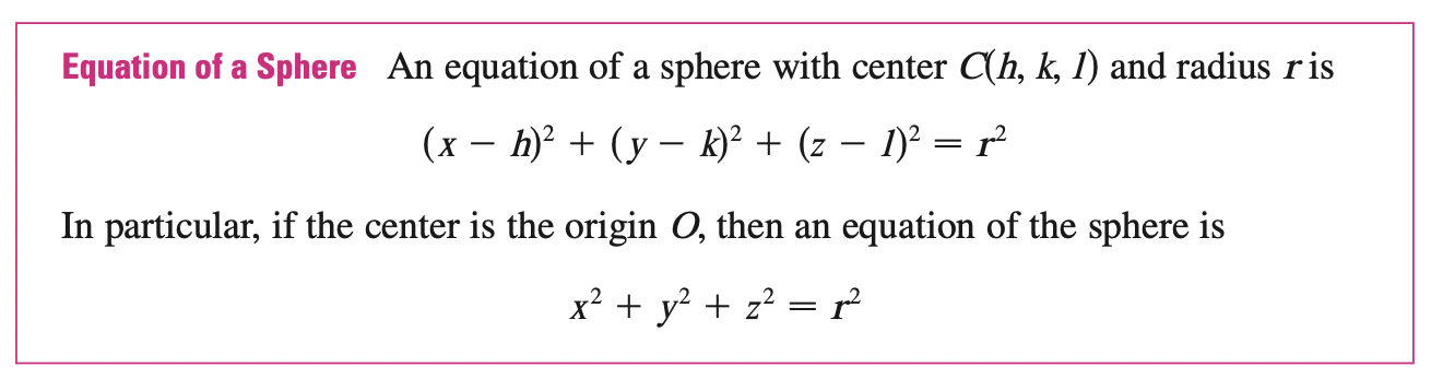
Equation of a sphere

By definition, a sphere is the set of all points \(P(x, y, z)\) whose distance from \(C\) is \(r\), where \(C\) is the center \(C(h, k, l)\). Thus, \(P\) is on the sphere if and only if

\[|PC| = r \implies |PC|^2 = r^2\]

\[(x - h)^2 + (y - k)^2 + (z - l)^2 = r^2\]

Dueling Network Architectures for Deep Reinforcement Learning

Introduction

The authors introduce an innovating neural network architecture that is better suited for model-free RL. This paper advances a new network but uses already published algorithms.

The proposed architecture is called dueling architecture, explicitly separates the representation of state values and state-dependent action advantages. The architecture consists of two streams that represent the value and advantage functions, while sharing a common convolutional feature learning module. The two streams are combined via a special aggregating layer to produce an estimate of the state-action value function \(Q\). This dueling network should be understood as a single Q network with two streams that replaces the popular single-stream Q-network in existing algorithms such as DQN. The dueling network automatically produces separate estimates of the state value function and advantage function, without any extra supervision.

Intuitively, the dueling architecture can learn which states are (or are not) valuable, without having to learn the effect of each action for each state. (by taking the gradient wrt to the input) It can more quickly identify the correct action during policy evaluation as redundant or similar actions are added to the learning problem.

Probability Background (2)

Distribution of Two Random Variables

Intuitive Example:

Let our experiment be flipping a coin 3 times. Then our sample space \(\Omega = \{HHH, THH, TTH, TTT, THT, HTH, HTT, HHT\}\). Let \(X_1\) be the number of head on the first two tosses and \(X_2\) be the number of heads on all three tosses. Then, our interest can be represented by the pair of random variables \((X_1, X_2)\), for example \((X_1 (HTH), X_2(HTH)) = (1, 2)\). Continuing this way, \(X_1, X_2\) are real-valued functions defined on the sample space \(\Omega\), which take the outcome and map from sample space to ordered number pairs: \[\mathbb{D} = \{(0, 0), (0, 1), (1, 1), (1, 2), (2, 2), (2, 3)\}\]

One the other hand, we can regard this ordered pair of functions as a vector function \(f: \Omega \rightarrow \mathbb{D} \subset \mathbb{R}^2\) defined by \(f(x) = <X_1(x), \; X_2(x)>, \quad x \in \Omega\).

We often denote random vectors using vector notations \(\mathbf{X} = (X_1, X_2)^{\prime}\) as a column vector.

Let \(\mathbb{D}\) be the range space of \((X_1, X_2)\). Let \(A\) be a subset of \(\mathbb{D}\). We can uniquely define the distribution of this random vector \(P_{X_1, X_2}\) in terms of the CDF:

\[F_{X_1, X_2} (x_1, x_2) = P_{X_1, X_2}((X_1 \leq x_1) \cap (X_2 \leq x_2)) = P_{X_1, X_2}(X_1 \leq x_1, \; X_2 \leq x_2)\]

For all \((x_1, x_2) \in \mathbb{R}^2\). At the same time:

\[P_{X_1, X_2}(a_1 < X_1 \leq b_1, \; a_2 < X_2 \leq b_2) = F_{X_1, X_2} (b_1, b_2) - F_{X_1, X_2} (a_1, b_2) - F_{X_1, X_2} (b_1, a_2) + F_{X_1, X_2} (a_1, a_2)\]

Hence, all induced probabilities can be formulated in terms of the cdf. We often call this cdf the joint cumulative distribution.

Probability Background (1)

Sets

A set is a collection of objects, which are the elements of set. If S is a set and \(x\) is an element of \(S\), we write \(x \in S\). If \(x\) is not an element of \(S\), we write \(x \notin S\). A set can have no elements, in which case it is called the empty set, denoted by \(\emptyset\).

Finite, Countable, Uncountable

If \(S\) contains a finite number of elements, say \(x_1, x_2, ..., x_n\), we write it as list of the elements in braces:

\[S = \{x_1, x_2, ...., x_n\}\]

if \(S\) contains countable infinitely many elements \(x_1, x_2, ...\), we can write:

\[S = \{x_1, x_2, ... \}\]

\(S\) is countable infinite, if the set is countable but has infinitely many elements. However, a set with uncountable elements can not be written down in a list.

We can denote set of all \(x\) that have certain property \(P\):

\[\{x | x \text{ satisfies } P\}\]

ie. the set of even integers can be written as \(\{k | k/2 \text{ is integer}\}\), \(\{x | 0 \leq x \leq 1\}\) (uncountable)

Learning From Stream of Data (Introduction)

In previous DP settings, we know the transition distribution \(P\) and reward distribution \(R\). Everything about the environment dynamics are given. However, in RL setting, we have no access to the environment dynamics, instead, we observe data from agent interacting with its environment.

A stream of data (rollout or trajectory):

\[X_1, A_1, R_1, X_2, A_2, R_2, ...\]

with \(A_t \sim \pi(\cdot | X_t), X_{t+1} \sim P(\cdot | A_t, X_t), X_1 \sim \rho(\cdot), R_t \sim R(\cdot | X_t, A_t)\)

The questions are:

1. How can we learn a value of a policy \(\pi\)?
2. How can we find the optimal policy \(\pi^{*}\)?

Double Q-learning

The Overestimation Phenomenon

Assume the agent observes during learning that action \(a\) and executed at state \(s\) resulting in the state \(s^{\prime}\) and some immediate reward \(r^{a}_{s}\). The Q-learning update can be written as:

\[Q(s, a) \leftarrow r^{a}_{s} + \gamma \max_{\hat{a}} Q(s^{\prime}, \hat{a})\]

It has been shown that repeated application of this update equation eventually yields \(Q\)-values that give rise to a policy which maximizes the expected cumulative discounted reward. However, these results only apply when \(Q-\)values are stored precisely. (e.g by a look up table)

Assume, instead, let \(Q\) be represented as a function approximator that induces some noise on the estimates of \(Q\). More specifically, let us assume that the current stored \(Q-\)values, denoted by \(Q^{approx}\), represent some implicit target values \(Q^{target}\), corrupted by a noise term \(Y^{\hat{a}}_{s^{\prime}}\), which is due to the function approximator:

\[Q^{approx} (s^{\prime}, \hat{a}) = Q^{target} (s^{\prime}, \hat{a}) + Y^{\hat{a}}_{s^{\prime}}\]

Here the noise is modeled by the family of random variable \(Y^{\hat{a}}_{s^{\prime}}\) with zero mean:

Clearly, the noise causes some error on the left-hand side.

Deep Reinforcement Learning with Double Q-Learning

Introduction

The authors show that the double Q-learning algorithm which was first proposed in a tabular setting, can be generalized to arbitrary function approximation, including DNN. They use this to construct a new algorithm called double DQN to solve the overestimation problem in DQN.

Notations

Define:

\[Q_{\pi} (s, a) = E[R_1 + \gamma R_2 + ... | S_0=s, A_0=a, \pi]\]

\[Q_{*} (s, a) = max_{\pi} Q_{\pi} (s, a)\]

\[\pi_{*} (s) = argmax_{a \in A} Q_{*} (s, a)\]

The Target:

\[Y_t^{Q} = R_{t+1} + \gamma max_{a} Q(S_{t+1}, a; \theta_{t})\]

A standard Q update using stochastic gradient decent is (Semi-gradient Q):

\[\theta_{t+1} = \theta_t + \alpha (Y_{t}^{Q} - Q(S_t, A_t; \theta_t)) \nabla_{\theta_t} Q(S_t, A_t; \theta_t)\]

Where \(\alpha\) is a scalar step size.

Deterministic Policy Gradient Algorithms

Introduction

In traditional policy gradient algorithms, policy is parametrized by a probability distribution \(\pi_{\theta} (a | s) = P[a | s; \theta]\) that stochastically selects action \(a\) in state \(s\) according to parameter vector \(\theta\). In this paper, the authors consider deterministic policies \(a = \mu_{\theta} (s)\).

From a practical viewpoint, there is a crucial difference between the stochastic and deterministic policy gradients. In the stochastic case, the policy gradient integrates over both state and action spaces, whereas in the deterministic case it only integrates over the state space:

\[E_{X\sim \rho^{\pi_\theta}A \sim \pi_{\theta}} [\nabla log \pi(A | X) Q^{\pi_{\theta}} (X, A)]\]

Thus, computing deterministic policies may require less samples.

An off-policy learning scheme is introduced here to ensure adequate exploration (i.e The basic idea is to choose actions according to a stochastic behaviour policy).

Policy Iteration

A different approach is based on the iterative application of:

1. Policy Evaluation: Given a policy \(\pi_k\), compute \(V^{\pi_k}, Q^{\pi_k}\)
2. Policy Improvement: Find a new policy \(\pi_{k+1}\) that is better than \(\pi_{k}\), i.e., \(V^{\pi_{k+1}} \geq V^{\pi_k}\) (with a strict inequality in at least one state, unless at convergence)

Value Iteration

VI is one of the fundamental algorithms for planning. Many RL algorithms are essentially the sample-based variants of VI (DQN). We directly use the results of fixed points proposition and contraction property of the Bellman operator we proved in Bellman Optimality Equations.

Idea

Starting from \(V_0 \in B(X)\), we compute a sequence of \((V_{k})_{k \geq 0}\) by:

\[V_{k+1} \leftarrow T^{\pi} V_{k}\]

By the contraction property of the Bellman operator and Uniqueness of fixed points proposition :

\[lim_{k \rightarrow \infty} \| V_k - V^{\pi}\|_{\infty} = 0\]

similar for \(Q\):

\[lim_{k \rightarrow \infty} \| Q_k - Q^{\pi}\|_{\infty} = 0\]