Linear Algebra (4)

Inner Product Spaces

If \(\lambda\) is a complex number, then we define \(\lambda \geq 0\) to be real number and nonnegative.

Inner Products and Norms

For \(z \in \mathbb{F}^n\), we define the norm of \(z\) w.r.t Euclidian inner product by:

\[\|z\| = \sqrt{|z_1|^2 + ... + |z_n|^2}\]

Where \(|z_1|^2 = z\bar{z} = a^2 + b^2\)

Definition 6.2: Dot Product

For \(x, y \in \mathbb{R}^n\), the dot product of \(x\) and \(y\), denoted \(x \cdot y\), is defined by:

\[x \cdot y = x_1y_1 + ... + x_ny_n\]

where \(x=(x_1, ..., x_n), y=(y_1, ..., y_n)\)

It has the following properties:

1. \(x \cdot x \geq 0, \; \forall x \in \mathbb{R}^n\)
2. \(x \cdot x = 0\) IFF \(x = 0\)
3. For \(y \in \mathbb{R}^n\) fixed, the map from \(\mathbb{R}^n \rightarrow \mathbb{R}\) that sends \(x \in \mathbb{R}^n\) to \(x \cdot y\) is linear.
4. \(x \cdot y = y \cdot x, \; \forall x, y \in \mathbb{R}^n\)

Linear Algebra (3)

Polynomials

Complex Conjugate and Absolute Value

Definition 4.2: \(Re(z)\), \(Im(z)\)

Suppose \(z = a + b_i\), where \(a\) and \(b\) are real numbers.

• The real part of \(z\), denoted \(Re(z)\), is defined by \(Re(z) = a\).
• The imaginary part of \(z\), denoted \(Im(z)\), is defined by \(Im(z) = b\).

Thus for every complex number \(z\), we have:

\[z = Re(z) + Im(z) i\]

Definition 4.3: Complex Conjugate, \(\bar{z}\), absolute value, |z|.

Suppose \(z \in \mathbb{C}\):

• The complex conjugate of \(z \in \mathbb{C}\), denoted \(\bar{z}\), is defined by: \[\bar{z} = Re(z) - Im(z)i\]
• The absolute value of a complex number \(z\), denoted \(|z|\), is defined by: \[|z| = \sqrt{(Re (z))^2 + (Im (z))^2}\]

Theorem 4.5: Properties of Complex Numbers

Suppose \(w, z \in \mathbb{C}\). Then:

• Sum of \(z\) and \(\bar{z}\): \[z + \bar{z} = 2 Re(z)\]
• Difference of \(z\) and \(\bar{z}\): \[z - \bar{z} = 2(Im (z)) i\]
• Product of \(z\) and \(\bar{z}\): \[z \bar{z} = |z|^2\]
• Additive and Multiplicative of Complex Conjugate: \[\overline{w + z} = \bar{w} + \bar{z}, \quad \overline{wz} = \bar{w}\bar{z}\]
• Conjugate of Conjugate: \[\bar{\bar{z}} = z\]
• Real and Imaginary Parts are Bounded by \(|z|\): \[|Re (z)| \leq |z|, \quad |Im(z)| \leq |z|\]
• Absolute Value of the Complex Conjugate: \[|\bar{z}| = |z|\]
• Multiplicative of Absolute Value \[|wz| = |w||z|\]
• Triangle Inequality: \[|w + z| \leq |w| + |z|\]

Linear Algebra (2)

Finite Dimensional Vector Space

Span and Linear Independence

List of vectors are written without surrounding parentheses. For example \((4, 1, 6), (9, 5, 7)\) is a list of length 2 of vectors in \(\mathbb{R}^3\).

Definition 2.3: Linear Combination

A linear combination of a list \(v_1, ..., v_m\) of vectors in \(V\) is a vector of the form:

\[a_1v_1 + ... + a_m v_m\]

where \(a_1, ..., a_m \in \mathbb{F}\)

\((17, -4, 2)\) is a linear combination of list of vectosr \((2, 1, -3), (1, -2, 4)\) with \(a_1 = 6, a_2=5\).

Definition 2.5: Span (Linear Span)

The set of all linear combinations of a list of vectors \(v_1, ..., v_m\) in \(V\) is called the span of \(v_1, ..., v_m\), denoted \(span(v_1, ..., v_m)\). In other words,

\[span(v_1, ..., v_m) = \{a_1v_1 + .... + a_m v_m; a_1, ..., a_m \in \mathbb{F}\}\]

The span of a list of vectors in \(V\) is the smallest subspace of \(V\) containing all the vectors in the list.

Real Analysis (4)

Sequences and Series of Functions [1]

Uniform Convergence of a Seuqence of Functions

Definition 6.2.1: Pointwise Convergence

For each \(n \in \mathbb{N}\), let \(f_n\) be a function defined on a set \(A \subseteq \mathbb{R}\). The sequence \((f_n)\) of functions converges pointwise on \(A\) to a function \(f\) if, for all \(x \in A\), the sequence of real numbers \(f_{n} (x)\) converges to \(f(x)\).

In this case, we write \(f_n \rightarrow f\), \(\lim_{n \rightarrow \infty} f_n = f\) or \(\lim_{n \rightarrow \infty} f_n(x) = f(x)\).

Definition 6.2.1B: Pointwise Convergence

Let \((f_n)\) be a sequence of functions defined on a set \(A \subseteq \mathbb{R}\). Then, \((f_n)\) convergence pointwise on \(A\) to a limit function \(f\) defined on \(A\) if, for every \(\epsilon > 0\) and \(x \in A\), there exists an \(N \in \mathbb{N}\) (perhaps depends on \(x\)) such that \(|f_{n} (x) - f(x) | < \epsilon\) whenever \(n \geq N\).

Definition 6.2.3: Uniform Convergence (Stronger than Pointwise)

Let \((f_n)\) be a sequence of functions defined on a set \(A \subseteq \mathbb{R}\). Then, \((f_n)\) convergence uniformly on \(A\) to a limit function \(f\) defined on \(A\) if, for every \(\epsilon > 0\), there exists an \(N \in \mathbb{N}\) such that \(|f_{n} (x) - f(x) | < \epsilon\) whenever \(n \geq N\) and \(x \in A\).

Similar to uniform continuous, this is a stronger, which involves finding \(N \in \mathbb{N}\) for a given \(\epsilon > 0\) for all \(x \in A\).

Graphically speaking, the uniform convergence of \(f_n\) to a limit \(f\) on a set \(A\) can be seen as there exists a point in the sequence after which each \(f_n\) is completely contained in the \(\epsilon\)-strip.

Linear Algebra (1)

All the notes precisely follows Linear Algebra Done Right by Sheldon Axler

Vector Spaces

Complex Numbers

Definition 1.1: Complex Numbers

1. A Complex Number is an order pair \((a, b)\), where \(a, b \in \mathbb{R}\).
2. Addition and multiplication is defined as: \[x + y = (a + b) + (c + d) = (a + c, b + d)\] \[xy = (a + b) (c + d) = (ac - bd, ad + bc)\]
3. \(i = (0, 1)\) and \(i^2 = (0, 1) (0, 1) = -1\)
4. Every complex number can be written as \[x = (a, b) = (a, 0) + (0, b) = (a, 0) + (b, 0)(0, 1) = a + bi\]
5. The set of all complex numbers is denoted by \(\mathbb{C}\): \[\mathbb{C} = \{a + bi: a, b \in \mathbb{R}\}\]
6. Addition and multiplication on \(\mathbb{C}\) are defined by \[(a + bi) + (c + di) = (a + c) + (b + d)i\] \[(a + bi) (c + di) = (ac - bd) + (ad + bc)i\]

\(a, c, b, d \in \mathbb{R}\)

If \(a \in \mathbb{R}\), we identify \(a + 0i\) with the real number \(a\). Thus we can think of \(\mathbb{R}\) as a subset of \(\mathbb{C}\).

Definition 1.2: Conjugate

If \(a, b\) are real and \(z = a + bi\), then the complex number \(\bar{z} = a - bi\) is called the conjugate of \(z\). The numbers \(a, b\) are the real part and the imaginary part of \(z\) respectively:

\[a = Re(z), \quad \quad b = Im(z)\]

Theorem 1.3A

If \(z\) and \(w\) are complex, then

1. \(\overline{z + w} = \bar{z} + \bar{w}\)
2. \(\overline{zw} = \bar{z}\bar{w}\)
3. \(z + \bar{z} = 2Re(z),\quad z - \bar{z} = 2i Im(z)\)
4. If \(z = a + bi\), \(z \bar{z} = a^2 + b^2\) is real and positive.
5. \(|z| = \sqrt{z\bar{z}} = \sqrt{a^2 + b^2}\) is unique.
6. \(|zw| = |z||w|\)

Real Analysis (3)

Basic Topology of \(\mathbb{R}\)

Open and Closed Sets

Definition 3.2.1: Open

A set \(O \subseteq \mathbb{R}\) is open if for all points \(a \in O\) there exists an \(\epsilon-neighborhood V_{\epsilon} (a) \subseteq O\).

\(\mathbb{R}\) is open \(\emptyset\) is open

Theorem 3.2.3

1. The union of an arbitrary collection of open sets is open.
2. The intersection of a finite collection of open sets is open.

Definition 3.2.4: Limit Point

A point \(x\) is a limit point of a set \(A\) if every \(\epsilon-neighborhood V_{\epsilon} (x)\) of \(x\) intersects the set \(A\) at some point other than \(x\). Limit points may not be in \(A\), consider the end points of open sets.

Theorem 3.2.5

A point \(x\) is a limit point of a set \(A\) if and only if \(x = \lim_{n \rightarrow \infty} a_n\) for some sequence \((a_n)\) contained in \(A\) satisfying \(a_n \neq x, \; \forall n \in \mathbb{N}\)

Definition 3.2.6: Isolated Point

A point \(a \in A\) is an isolated point of \(A\) if it is not a limit point of \(A\). Isolated point is always in \(A\).

Definition 3.2.7: Closed Set

A set \(F \subseteq \mathbb{R}\) is closed if it contains all its limit points. Topologically speaking, a closed set is one where convergent sequences within the set have limits that are also in the set.

Real Analysis (2)

Sequence

The Limit of Sequence

Definition 2.2.1: Definition of Sequence

A sequence is a function whose domain is \(\mathbb{N}\). Given a function \(f: \mathbb{N} \rightarrow \mathbb{R}\), \(f(n)\) is just the \(n\)th term on the list.

\((1, \frac{1}{2}, \frac{1}{3}...)\) is a sequence: \[f(n) = \{n \in \mathbb{N}: \frac{1}{n}\}\]

Definition 2.2.3: Convergence of a Sequence

A sequence \((a_n)\) converges to a real number \(a\) if, for every positive number \(\epsilon\), there exists an \(N \in \mathbb{N}\) such that whenever \(n \geq \mathbb{N}\), it follows that \(|a_n - a| < \epsilon\).

\[\lim_{n \rightarrow \infty} a_n = a\]

Definition 2.2.4

Given a real number \(a \in \mathbb{R}\) and a positive number \(\epsilon > 0\), the set:

\[V_{\epsilon} (a) = \{x \in \mathbb{R}: |x - a| < \epsilon\}\]

is called the \(\boldsymbol{\epsilon-neighborhood}\) of \(a\). In other words, \(V_{\epsilon} (a)\) is an interval, centered at \(a\), with radius \(\epsilon\).

Definition 2.2.3B

A sequence \((a_n)\) converges to \(a\) if, given any \(\epsilon-neighborhood V_{\epsilon}(a)\) of \(a\), there exists a point in the sequence after which all of the terms are in \(V_{\epsilon} (a)\).

Real Analysis (1)

Preliminaries

Sets

If an element \(x\) is in a set \(A\), we write:

\[x \in A\]

and say that \(x\) is a member of \(A\), or that \(x\) belongs to \(A\). If \(x\) is not in \(A\), we write:

\[x \notin A\]

If every element of a set \(A\) also belongs to a set \(B\), we say that \(A\) is a subset of \(B\) and write:

\[A \subseteq B\]

We say that \(A\) is a proper subset of \(B\) if \(A \subset B\), but there is at least one element of \(B\) that is not in \(A\). In this case we write:

\[A \subset B\]

Definition 1.11: Equal Sets

Two sets \(A\) and \(B\) are said to be equal, we write \(A = B\) if they contain the same elements. Thus, to prove that sets \(A\) and \(B\) are equal, we must show that:

\[A \subseteq B, \;\; B \subseteq A\]

A set is normally defined by either listing its elements explicitly, or by specifying a property that determines the elements of the set. If \(P\) denotes a property that is meaningful and unambiguous for elements of a set \(S\), then we write:

\[\{x \in S; P(x)\}\]

for the set of all elements \(x\) in \(S\) for which the property \(P\) is true.

Attention is all you need

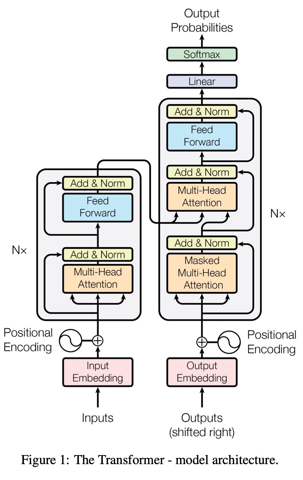
Structure

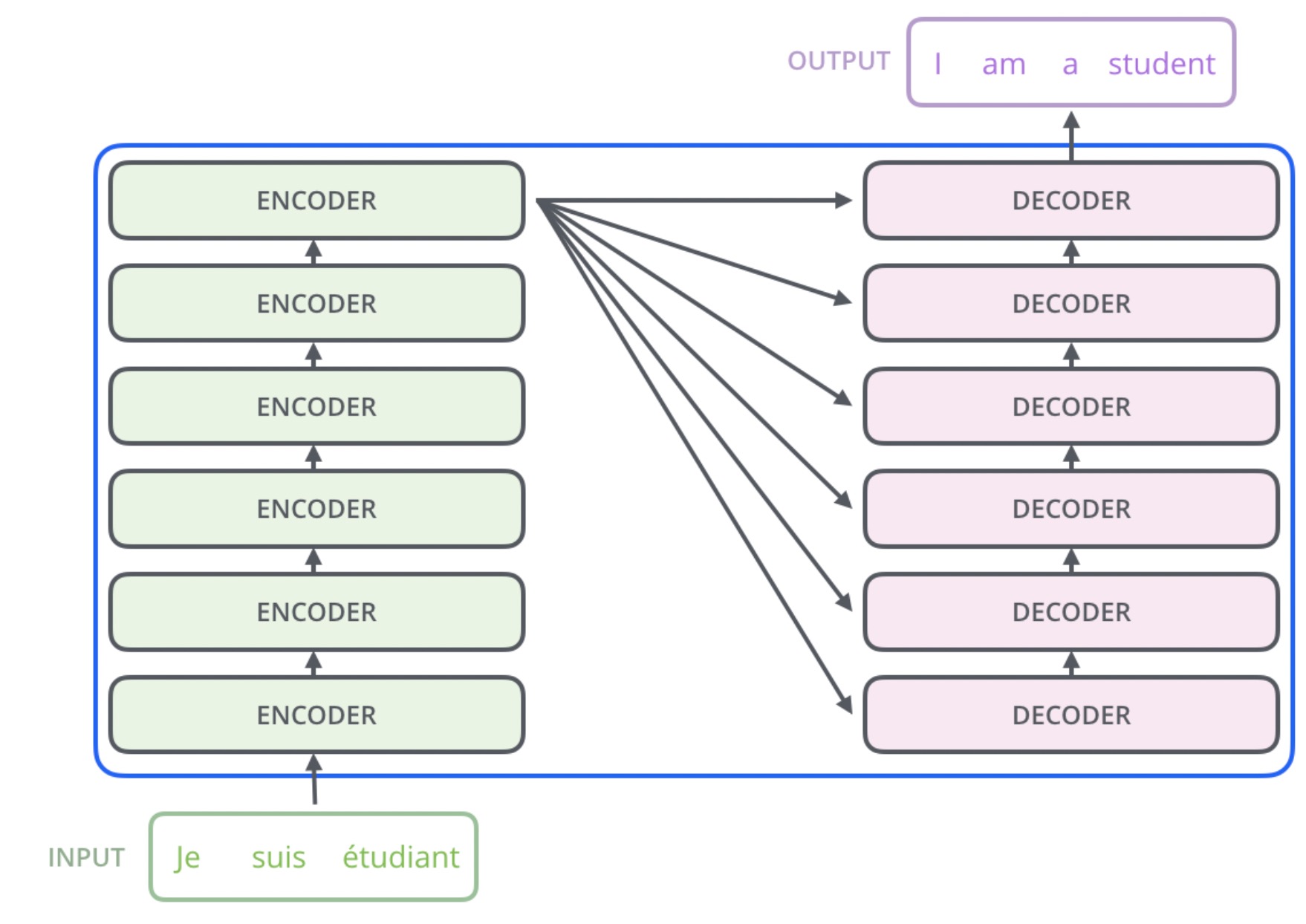
Encoder

The encoder consists of 6 identical layers. Each layer consists of two sub-layers: 1. Multihead self-attention 2. Feed forward fully connected network

residual connection (skip connection) are employed around each of the two sub-layers followed by layer normalization. The output of each sub-layer is:

\[\text{LayerNorm}(x + \text{Sublayer}(x))\]

Where \(\text{Sublayer}(x)\) is the function implemented by the sub-layer itself. All sub-layers and embedding layers have output of dimension \(d_{model} = 512\)

Decoder

The decoder consists of 6 identical layers. In addition to the two sub-layers in each encoder layer, the decoder inserts a third sub-layer, which performs multi-head attention over the output of the encoder stack as key, value and the previous decoder output as query. The first self-attention sub-layer is modified to mask the future during training, this ensures that the predictions for position \(i\) can depend only on the known outputs at positions less than \(i\).

Self Attention

Given input \(X \in \mathbb{R}^{n_b \times n_s \times d_{model}}\) and trainable parameters \(W_q \in \mathbb{R}^{d_{model} \times d_{k}}, W_k \in \mathbb{R}^{d_{model} \times d_{k}}, W_v \in \mathbb{R}^{d_{model} \times d_{v}}\), matrices query \(Q \in \mathbb{R}^{n_b \times n_s \times d_k}\), key \(K \in \mathbb{R}^{n_b \times n_s \times d_k}\), value \(V \in \mathbb{R}^{n_b \times n_s \times d_v}\) are defined as:

\[Q = XW_q, \;\; K = XW_k, \;\; V = XW_v\]

Scaled Dot-Product Attention

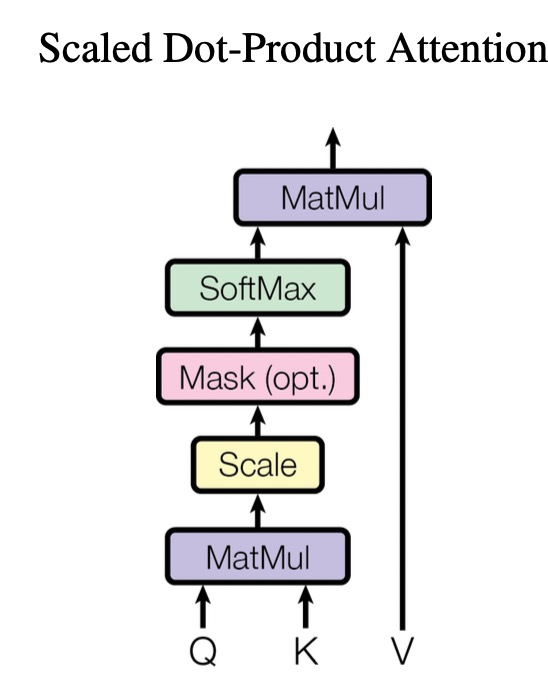
\[\text{Attention}(Q, K, V) = \text{softmax}(\frac{QK^T}{\sqrt{d_k}}) V\]

The scale is used to prevent the large magnitude of the dot product so that the gradient of softmax vanishes.

Multi-head Self Attention

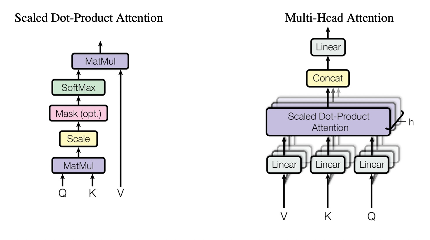
Instead of using a single attention function, \(h\) of parallel attention functions with different \(W^q_i, W^k_i, W^v_i\) are used and concatenated into single self attention matrix. The final self attention matrix is then multiplied by a weight matrix \(W_o \in \mathbb{R}^{hd_v \times d_{model}}\):

\[\text{MultiHead} (Q, K, V) = \text{Concat} (\text{head}_1, ...., \text{head}_h) W_o\]

Where

\[\text{head}_i = \text{Attention}(QW^Q_i, KW^k_i, VW^V_i)\]

In this paper \(h = 8, d_{model} = 512, d_{model} / h = d_k = d_v = 64\) and in a multi-head self-attention layer, all the keys, values and queries come from same place which is the output of the previous layer in the encoder. (i.e \(Q = K = V = X\) where \(X\) is the output from previous layer)

Position-wise Feed-Forward Networks

In addition to attention sub-layers, each of the layers in the encoder and decoder contains a fully connected feed-forward network. This consists of two linear transformations with a ReLU activation in between:

\[\text{FFN}(\mathbf{x}) = max(0, \mathbf{x} W_1 + \mathbf{b}_1) W_2 + \mathbf{b}_2\]

The parameters are different for different layers. The dimensionality of input and output is \(d_{model} = 512\), and the inner-layer has dimensionality \(d_{ff} = 2048, W_1 \in \mathbb{R}^{502 \times 2048}, W_2 \in \mathbf{2048 \times 502}\)

Positional Encoding

Since the model contains no recurrence and no convolution, in order for the model to make use of the order of the sequence, we must inject some information about the relative or absolute position of the tokens in the sequence. Thus, we add positional encodings to the input embeddings at the bottoms of the encoder and decoder stacks. The positional encodings have the same dimension \(d_{model}\) as the embeddings, so that the two can be summed:

\[PE_{(pos, 2i)} = \sin(\frac{pos}{10000^{\frac{2i}{d_{model}}}})\] \[PE_{(pos, 2i+1)} = \cos(\frac{pos}{10000^{\frac{2i}{d_{model}}}})\]

Where \(i\) is the dimension, \(pos\) is the position. For example \(PE(1) = [\sin(\frac{1}{10000^{\frac{0}{d_{model}}}}), \cos(\frac{1}{10000^{\frac{2}{d_{model}}}}), \sin(\frac{1}{10000^{\frac{4}{d_{model}}}}) ....]\)

It has several properties:

1. For each time-step, it outputs a unique encoding.
2. The distance between two time-steps is consistent across sentences with different lengths.
3. Deterministic
4. \(PE_{pos+k}\) can be represented linearly using \(PE_{pos}\), so it generalizes easily to unseen length sequences.

Ref

https://jalammar.github.io/illustrated-transformer/

https://theaisummer.com/self-attention/

https://zhuanlan.zhihu.com/p/98641990

https://kazemnejad.com/blog/transformer_architecture_positional_encoding/#the-intuition

Temporal Convolutional Networks

Characteristics of TCN:

1. The convolutions in the architecture are causal.
2. The architecture can take a sequence of any length and map it to an output sequence of same length.
3. The ability of long term memories using a combination of very deep networks (with residual layers) and dilated convolutions.

Fully Convolutional Network

Fully convolutional networks replace the fully connected layers with convolution layers. The TCN uses a \(1D\) fully-convolutional network architecture, where each hidden layer is the same length as the input layer and zero padding of length (kernel - 1) in the front of the sequence is added to keep subsequent layers the same length as previous ones.

Causal Convolutions

To achieve the causality, the TCN uses causal convolutions, convolutions where an output at time \(t\) is convolved only with elements from time \(t\) and earlier in the previous layer. Thus:

\[\text{TCN} = 1D\text{FCN} + \text{causal convolutions}\]

The major disadvantage of this design is that we need an extremely deep network or very large filters to achieve a long effective history size.

Dilated Convolutions

The solution is to introduce dilated convolutions:

\[F_d(\mathbf{x}, s) = \sum^{k-1}_{i=0} f(i) \cdot \mathbf{x}_{s - d\cdot i}\]

Where \(f(i)\) is the \(i\)th component of the 1D filter with length \(k - 1, i=0, ...., k-1\) and \(d\) is the dilation factor, \(k\) is the filter size, and \(s - d \cdot i\) accounts for the direction of the past. Using large dilation enables an output at the top level to represent a wider range of inputs, thus effectively expanding the receptive field of a ConvNet. Thus, we can choose to: 1. Larger filter size \(k\). 2. Choose larger Dilation factor \(d\). Usually it is increased exponentially with the depth of the network \(d = 2^i\) at level \(i\) of the network. This ensures that there is some filter that hits each input within the effective history, while also allowing for an extremely large effective using deep networks.

Residual Connections

To allow faster learning , a residual block is introduced with weight norm and dropout inbetween to replace the convolution layer:

In TCN, the input and output of the residual block could have different widths (channels), to account for discrepant input-output widths, we use an additional \(1 \times 1\) convolution to ensure that elementwise addition will work.

Advantages of TCN

1. Parallelism:
2. Flexible Receptive Field Size
3. Stable Gradients
4. Low Memory Requirement for Training
5. Variable length inputs

Disadvantages of TCN

1. Data storage during evaluation:
2. Potential parameter change for a transfer of domain: