Time Series (ARIMA)

Autoregressive Moving Average Models (ARMA)

Autoregressive Models

Autoregressive models are based on the idea that the current value of the series \(X_t\) can be explained as a function of \(p\) past values, \(X_{t-1}, X_{t-2}, ..., X_{t-p}\) where \(p\) determines the number of steps into the past needed to forecast the current value.

An autoregressive model of order \(p\), abbreviated \(AR(p)\) with \(E[X_t] = 0\), is of the form:

\[X_t = \phi_1 X_{t-1} + \phi_2 X_{t-2} + ... + \phi_p X_{t-p} + W_t\]

Where \(X_t\) is stationary, \(\phi_1, ..., \phi_p \neq 0\) are constants, \(W_t\) is a Gaussian white noise series with mean zero and variance \(\sigma^2_w\). We assume above equation \(X_t\) has mean zero, if it has non zero mean \(\mu\), we can replace it by:

\[X_t - \mu = \phi(X_{t-1} - \mu) + \phi_2(X_{t-2} - \mu) + ... + \phi_p (X_{t-p} - \mu) + W_t\] \[\implies X_t = \alpha + \phi_1 X_{t-1} + \phi_2 X_{t-2} + ... + \phi_p X_{t-p} + W_t\]

Where \(\alpha = \mu(1 - \phi_1 - ... - \phi_p)\).

We can also use the backshift operator to rewrite the zero mean \(AR(p)\) process as:

\[(1 - \phi_1 B - \phi_2 B^2 - ... - \phi_p B^p) X_t = W_t\]

or using autoregressive operator:

\[\phi(B)X_t = W_t\]

Time Series (Introduction)

Characteristics of Time Series

The primary objective of time series analysis is to develop mathematical models that provide plausible descriptions for sample data with time correlations. In order to provide a statistical setting for describing the character of data that seemingly fluctuate in a random fashion over time, we assume a time series can be defined as a collection of random variables indexed according to the order they are obtained in time. In general, a collection of random variables \(\{X_t\}\) indexed by \(t\) is referred to as a stochastic process. In this text, \(t\) will typically be discrete and vary over the integers.

Example of Series:

White Noise: A collection of uncorrelated, independent and identically distributed random variables \(W_t\) with mean 0 and finite variance \(\sigma^2_w\). A particular useful white noise is Gaussian white noise, that is \(W_t \overset{i.i.d}{\sim} N(0, \sigma^2_w)\)

Moving Average: We might replace the white noise series \(W_t\) by a moving average that smooths the series: \[V_t = \frac{1}{3} (W_{t-1} + W_{t} + W_{t+1})\] This introduces a smoother version of white noise series, reflecting the fact that the slower oscillations are more apparent and some of the faster oscillations are taken out.

Autoregressions: Suppose we consider the white noise series \(W_t\) as input and calculate the output using the second-order equation: \[X_t = X_{t-1} - 0.9 X_{t-2} + W_t\] For \(t=1, ..., 500\). We can see the periodic behavior of the series.

Sequential Data

In some cases, we have i.i.d assumptions to allow use to express the likelihood function as the product over all data points of the probability distribution evaluated at each data point. However, in some cases namely sequential data, we may not have i.i.d samples.

Markov Models

To express the sequential dependence of the samples, we can relax the i.i.d assumption and one of the simplest ways to do this is to consider a Markov Model. First of all, without loss of generality, we can use the product rule to express the joint distribution for a sequence of observations in the form:

\[P(X_1, ...., X_n) = \prod^N_{n=1} P(X_n | X_1, ..., X_{n-1})\]

If we assume that each of the conditional distributions on the right-hand side is independent of all previous observations except the most recent, we obtain the first-order Markov Chain, which can depicted as graphical model:

The joint distribution for a sequence of \(N\) observations under this model is given by:

\[P(X_1, ..., X_N) = P(X_1) \prod^{N}_{n=2} P(X_n | X_{n-1})\]

Thus, if we use such a model to predict the next observation in a sequence, the distribution of predictions will depend only on the value of the immediately preceding observation and will be independent of all earlier observations. In most applications of such models, the conditional distributions \(P(X_n | X_{n-1})\) that define the model will be constrained to be equal, corresponding to a assumption of a stationary time series. The model is then known as the homogeneous Markov Chain (All conditional distribution share the same parameters).

However, first-order Markov model is still restrictive. For many sequential observations, we anticipate that the trends in the data over several successive observations will provide important information in predicting the next value. One way to allow earlier observations to have an influence is to move to higher-order Markov chains, the second-order Markov chain is given by:

\[P(X_1, ..., X_N) = P(X_1) P(X_2 | X_1) \prod^{N}_{n=3} P(X_n | X_{n-1}, X_{n-2})\]

Suppose we wish to build a model for sequences that is not limited by the Markov assumption to any order and yet that can be specified using a limited number of free parameters. We can achieve this by introducing additional latent variables to permit a rich class of models to be constructed out of simple components, as we did with mixture distributions.

For each observation \(\mathbf{X}_n\), we introduce a corresponding latent random vector \(\mathbf{Z}_n\) which may be of different type or dimensionality to the observed variable. We now assume that it is the latent variables that form a Markov chain, giving rise to the graphical structure known as state space model. It satisfies the key conditional independence properties that \(\mathbf{Z}_{n-1}, \mathbf{Z}_{n+1}\) are independent given \(\mathbf{Z}_n\) so that:

\[\mathbf{Z}_{n+1} \perp \!\!\! \perp \mathbf{Z}_{n-1} \;|\; \mathbf{Z}_n\]

The joint distribution of the model is:

\[P(\mathbf{X}_1, ...., \mathbf{X}_{N}, \mathbf{Z}_1, ...., \mathbf{Z}_{N}) = P(\mathbf{Z}_1) \prod^N_{n=1} P(\mathbf{X}_n | \mathbf{Z}_n) \prod^{N}_{n=2} P(\mathbf{Z}_n | \mathbf{Z}_{n-1})\]

Using the d-separation criterion, we see that there is always a path connecting any two observed variables \(\mathbf{X}_n\) and \(\mathbf{X}_{n+1}\) via the latent variable, so the predictive distribution \(P(\mathbf{X}_{n+1} | \mathbf{X}_{1} , ..., \mathbf{X}_{n})\) does not have any conditional dependence properties so it depends on all previous variables.

There are two important models for sequential data:

1. Hidden Markov Model: If the latent variables are discrete.
2. Linear Dynamical System: If the latent variables, observed variables are Gaussian with a linear-Gaussian dependence of the conditional distributions on their parents.

Hidden Markov Models

The hidden markov model can be viewed as specific instance of the state space model with discrete latent variables. It can also be viewed as an extension of a mixture model in which the choice of mixture component for each observation is not selected independently but depends on the choice of component for the previous observation.

It is convenient to use 1-of-\(K\) coding scheme for the latent variables \(\mathbf{Z}_n\). We now allow the probability distribution of \(\mathbf{Z}_n\) to depend on the state of previous latent variable \(\mathbf{Z}_{n-1}\) through a conditional probability distribution \(P(\mathbf{Z}_{n} | \mathbf{Z}_{n-1})\). Since, we want to express the dependency of each element of \(\mathbf{Z}_n\) on each element of \(\mathbf{Z}_{n-1}\), we introduce a \(K \times K\) matrix of probabilities that we denote by \(\mathbf{A}\), the element of which are known as transition probabilities:

\[A_{jk} = P(Z_{nk} = 1 | Z_{n-1, j}) = 1\]

And because they are probabilities:

\[\sum^K_{k=1} A_{jk} = 1\]

\[0 \geq A_{jk} \leq 1\]

We can write the conditional distribution explicitly in the form:

\[P(\mathbf{Z}_{n} | \mathbf{Z}_{n-1}, \mathbf{A}) = \prod^K_{k=1}\prod^{K}_{j=1} A_{jk}^{Z_{nk}Z_{n-1, \;j}}\]

The initial latent node \(\mathbf{Z}_1\) is special in that it does not have a parent node, and so it has a marginal distribution \(P(\mathbf{Z}_1)\) represented by a vector of probabilities that represents the initial probabilities \(\boldsymbol{\pi}\):

\[\pi_k = P(Z_{1k} = 1)\] \[\sum^{K}_{k=1} \pi_k = 1\] \[P(\mathbf{Z}_1 | \boldsymbol{\pi}) = \prod^K_{k=1} \pi_k^{Z_{1k}}\]

Lastly, the specification of the probabilistic model is completed by defining the conditional distribution of observed variables \(P(\mathbf{X}_n | \mathbf{Z}_n, \boldsymbol{\phi})\), where \(\boldsymbol{\phi} = \{\boldsymbol{\phi}_1, ...., \boldsymbol{\phi}_K\}\) is a set of parameters governing the distribution. These distributions are called emissino distribution and might be given by Gaussian if the elements of \(\mathbf{X}\) are continues random variables or by conditioanl probability tables if \(\mathbf{X}\) are discrete. Since the distribution depends on the values of \(\mathbf{Z}\) which has \(K\) possible states, We can define the emission distribution as:

\[P(\mathbf{X}_n | \mathbf{Z}_n, \boldsymbol{\phi}) = \prod^K_{k=1} P(\mathbf{X}_n | \boldsymbol{\phi}_k)^{Z_{nk}}\]

In this case, we focus on Homogeneous models for which all the conditional distributions governing the latent variables share the same parameters \(\mathbf{A}\) and similarly all of the emission distributions share the same parameters \(\boldsymbol{\phi}\), so the joint distribution is:

\[P(\mathbf{X}_1, ...., \mathbf{X}_{N}, \mathbf{Z}_1, ...., \mathbf{Z}_{N} | \boldsymbol{\theta}) = P(\mathbf{D}, \mathbf{H} | \boldsymbol{\theta}) = P(\mathbf{Z}_1 | \boldsymbol{\pi}) \prod^N_{n=1} P(\mathbf{X}_n | \mathbf{Z}_n, \boldsymbol{\phi}) \prod^{N}_{n=2} P(\mathbf{Z}_n | \mathbf{Z}_{n-1}, \mathbf{A})\]

Where \(\boldsymbol{\theta} = \{\boldsymbol{\pi}, \boldsymbol{\phi}, \boldsymbol{A}\}\)

Maximum Likelihood for HMM

If we have observed a dataset \[\mathbf{D} = \{\mathbf{x}_1, ...., \mathbf{x}_N\}\], we can determine the parameters of an HMM using maximum likelihood method. The likelihood function is obtained from the joint distribution by marginalizing over the latent variables:

\[L(\boldsymbol{\theta} ;\; \mathbf{D}) = \sum_{\mathbf{H}} P(\mathbf{D}, \mathbf{H} | \; \boldsymbol{\theta}) = P(\mathbf{D} | \; \boldsymbol{\theta}) = \prod^N_{n=1} P(\mathbf{x}_n |\; \boldsymbol{\theta})\]

This is similar to the mixture distribution with latent variable in EM, we have a summation inside the log for log likelihood which is much difficult to work with, direct maximization of the log likelihood function will therefore lead to complex expressions with no closed-form solutions. Thus, one way to solve the problem is to use EM algorithm to find an efficient framework for maximizing the likelihood function in HMM.

The EM algorithm starts with some initial selection for the model parameters, which we denote by \(\boldsymbol{\theta}^{old}\):

1. E step:
   • We take these parameter values and find the posterior distribution of the latent variables: \[P(\mathbf{H} | \mathbf{X}, \boldsymbol{\theta}^{old})\]
   • We then evaluate the expectation of complete log likelihood function over the posterior distribution of the latent variables as a function of new parameters \(\boldsymbol{\theta}\): \[Q(\boldsymbol{\theta}, \boldsymbol{\theta}^{old}) = E_{\mathbf{H} | \mathbf{D}, \boldsymbol{\theta}^{old}}[\ln P(\mathbf{D}, \mathbf{H} | \boldsymbol{\theta}) | \mathbf{D}, \boldsymbol{\theta}^{old}]\]
   • We can rewrite the log likelihood as: \[\begin{aligned} Q(\boldsymbol{\theta}, \boldsymbol{\theta}^{old}) &= \sum_{\mathbf{H}} P(\mathbf{H} | \mathbf{D}, \boldsymbol{\theta}^{old}) \ln P(\mathbf{D}, \mathbf{H} | \boldsymbol{\theta})\\ &= \sum^{K}_{k=1}P(Z_{1k} = 1 | \mathbf{D}, \boldsymbol{\theta}^{old}) \ln P(Z_{1k} = 1| \boldsymbol{\pi}) + \sum^N_{n=2}\sum^{K}_{j=1}\sum^{K}_{k=1} P(Z_{nk}, Z_{n-1, j} | \mathbf{D}, \boldsymbol{\theta}^{old}) \ln P(Z_{nk} | Z_{n-1, j}) + \sum^{N}_{n=1}\sum^{K}_{k=1} P(Z_{nk} = 1 | \mathbf{D}, \boldsymbol{\theta}^{old}) \ln P(\mathbf{X}_n| \boldsymbol{\phi}_k, Z_{nk}=1)\\ &= \sum^{K}_{k=1} \gamma(Z_{nk})\ln \pi_k + \sum^N_{n=2}\sum^{K}_{j=1}\sum^{K}_{k=1} \xi(Z_{nk}, Z_{n-1, j})\ln A_{jk} + \sum^{N}_{n=1}\sum^{K}_{k=1} \gamma(Z_{nk}) \ln P(\mathbf{X}_n| \boldsymbol{\phi}_k, Z_{nk}=1) \end{aligned}\] Where \(\gamma (Z_{nk}) = P(Z_{1k} = 1 | \mathbf{D}, \boldsymbol{\theta}^{old})\) and \(\xi(Z_{nk}, Z_{n-1, j}) = P(Z_{nk}, Z_{n-1, j} | \mathbf{D}, \boldsymbol{\theta}^{old}) \ln P(Z_{nk} | Z_{n-1, j})\)
   • Our goal is to evaluate these posterior probabilities \(\gamma, \xi\) efficiently
2. M step:
   • We maximize \(Q(\boldsymbol{\theta}, \boldsymbol{\theta}^{old})\) w.r.t the parameters \(\boldsymbol{\theta}\) in which we treat posterior probabilities as constant:

Ref

PRML Chapter 13

Variational Inference

Graphical Models

Conditional Independence

Conditional Independence of Random Variable

Let \(\mathbf{X}, \mathbf{Y}, \mathbf{Z}\) be a set of random variables. We say that \(\mathbf{X}\) is conditionally independent of \(\mathbf{Y}\) given \(\mathbf{Z}\) in a distribution \(P\) if \(P\) satisfies \(P(\mathbf{X} = x \perp \mathbf{Y}=y | \mathbf{Z}=z)\) for all values of \(x, y, z \in (Val(\mathbf{X}), Val(\mathbf{Y}), Val(\mathbf{Z}))\). If the set \(\mathbf{Z}\) is empty, we write \((\mathbf{X} \perp \mathbf{Y})\) and say that \(\mathbf{X}\) and \(\mathbf{Y}\) are marginally independent.

The distribution \(P\) satisfies \((\mathbf{X} \perp \mathbf{Y} | \mathbf{Z})\) IFF \(P(\mathbf{X}, \mathbf{Y} | \mathbf{Z}) = P(\mathbf{X}| \mathbf{Z}) P(\mathbf{Y} | \mathbf{Z})\)

• Symmetry: \[(\mathbf{X} \perp \mathbf{Y} | \mathbf{Z}) \implies (\mathbf{Y} \perp \mathbf{X} | \mathbf{Z})\]
• Decomposition: \[(\mathbf{X} \perp \mathbf{Y}, \mathbf{W} | \mathbf{Z}) \implies (\mathbf{X} \perp \mathbf{Y} | \mathbf{Z}), \;(\mathbf{X} \perp \mathbf{W} | \mathbf{Z})\]
• Weak Union: \[(\mathbf{X} \perp \mathbf{Y}, \mathbf{W} | \mathbf{Z}) \implies (\mathbf{X} \perp \mathbf{Y} | \mathbf{Z}, \mathbf{W}), \; (\mathbf{X} \perp \mathbf{W} | \mathbf{Z}, \mathbf{Y})\]
• Contraction: \[(\mathbf{X} \perp \mathbf{W} | \mathbf{Z}, \mathbf{Y}) \cap (\mathbf{X} \perp \mathbf{Y} | \mathbf{Z}) \implies (\mathbf{X} \perp \mathbf{Y}, \mathbf{W}| \mathbf{Z})\]

We can represent complicated probabilistic models using diagrammatic representations of probability distributions called probabilistic graphical models. These offer several useful properties:

1. They provide a simple way to visualize the structure of a probabilistic model and can be used to design and motivate new models.
2. Insights into the properties of the model, including conditional independence properties can be obtained by inspection of the graph.
3. Complex computations, required to perform inference and learning in sophisticated models, can be expressed in terms of graphical manipulations, in which underlying mathematical expressions are carried along implicitly.

A probabilistic graphical model consists of:

1. Nodes: each random variable (or group of random variables) is represented as a node in the graph
2. Edges (links): links express probabilistic relationship between these random variables, the edges encode our intuition about the way the world works.
   • Directed graphical models: in which the edges of the graphs have a particular directionality indicated by arrows (Bayesian networks). Directed graphs are useful for expressing causal relationships between random variables.
   • Undirected graphical models: in which the edges of the graph do not carry arrows and have no directional significance (Markov random fields). Undirected graphs are better suited to expressing soft constraints between random variables.

The graph then captures the way in which the joint distribution over all of the random variables can be decomposed into a product of factors each depending only on a subset of the variables.

Bayesian Networks

The DAG of random variables can be viewed in two very different ways (Also strongly equivalent):

• As a data structure that provides the skeleton for representing a joint distribution compactly in a factorized way.
• As a compact representation for a set of conditional independence assumptions about a distribution.

We can view the graph as encoding a generative sampling process executed by nature, where the value for each variable is selected by nature using a distribution that depends only on its parents. In other words, each variable is a stochastic function of its parents.

In general, there are many weak influences that we might choose to model, but if we put in all of them, the network can become very complex, such networks are problematic from a representational perspective.

Bayesian Network Represents a Joint Distribution Compactly in a Factorized Way

Consider first an arbitrary joint distribution defined by \(P(\mathbf{Z})\) over random vector \(\mathbf{Z} = <A, B, C>\), by product rule, we have:

\[P(\mathbf{Z}) = P(C| A, B) P(A, B) = P(C | A, B) P(B | A) P(A)\]

We now represent the right-hand side in terms of a simgple graphical model as follows:

1. First, we introduce a node for each of the random variables \(A, B, C\) and associate each node with the corresponding conditional distribution on the right-hand side.
2. Then, for each conditional distribution we add directed links to the graph from the nodes to the variables on which the distribution is conditioned.

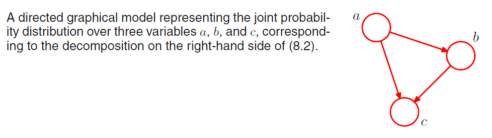
If there is a link going from a node \(A\) to a node \(B\), then we say that node \(A\) is parent of node \(B\) and \(B\) is the child of node \(A\) (change ordering of the decomposition will change the graph).

We can extend the idea to joint distribution of \(K\) random variables given by \(P(X_1, ...., X_K)\). By repeated application of the product rule of the probability, this joint distribution can be written as a product of conditional distributions:

\[P(X_1, ...., X_K) = P(X_K | X_{K-1}, ..., X_{1}) ... P(X_2 | X_1) P(X_1)\]

We can generate a graph similar to three-variable case, each node having incoming links from all lower numbered nodes. We say this graph is fully connected because there is a link between every pair of nodes. However, it is the absence (not fully connected) of links in the graph that conveys interesting information about the properties of the class of distributions that the graph represents.

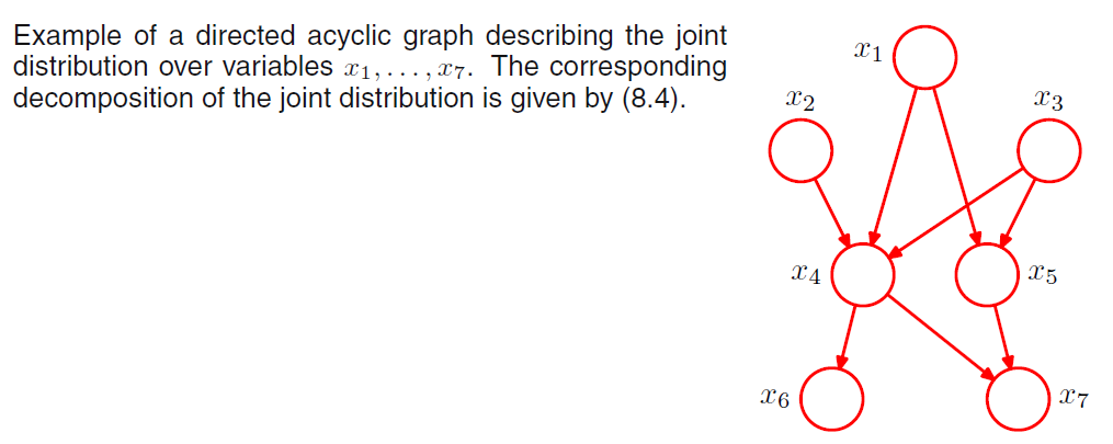
We can now state in general terms the relationship between a given directed graph and the corresponding distribution over the variables. Thus, for a graph with K nodes \(\mathbf{X} = <X_1, ...., X_K>\), the joint distribution is given by:

\[P(\mathbf{X}) = \prod^K_{k=1} P(X_k | \text{Parent}(X_k))\]

Where \(\text{Parent}(X_k)\) denotes the set of parents of \(X_k\).

Notice that, the directed graphs that we are considering are subject to an important restriction namely that there must be no directed cycles, that is, we are working with directed acyclic graphs or DAGs.

Example: Generative Models

There are many situations in which we wish to draw samples from a given probability distribution. One technique which is particularly relevant to graphical models is called ancestral sampling.

Consider a joint distribution \(P(\mathbf{X}), \mathbf{X} = <X_1, ...., X_K>\) that factorizes into a DAG. We shall suppose that the variables have been ordered from \(X_1\) to \(X_K\), in other words each node has a higher index than any of its parents. Our goal is to draw samples \(\hat{X}_1, ..., \hat{X}_K\) from the joint distribution.

To do this, we start from \(X_1\), and draw sample \(\hat{X}_1\) from the distribution \(P(X_1)\). We then work through each of the nodes in order, so that for node \(n\) we draw a sample from the conditional distribution \(P(X_n | \text{Parent}(X_n))\), in which the parent variables have been set to their sampled values.

To obtain a sample from some marginal distribution corresponding to a subset of the random variables, we simply take the sampled values for the required nodes and discard the rest. For example, to draw a sample from the distribution \(P(X_2, X_4)\), we simply sample from the full joint distribution and then retain the values \(\hat{X}_2, \hat{X}_4\) and discard the remaining values.

For practical applications of probabilistic models, it will typically be the higher-numbered variables corresponding to terminal nodes of the graph that represent the observations, with lower-numbered nodes corresponding to latent variables. The primary role of the latent variables is to allow a complicated distribution over the observed variables to tbe represented in terms of a model constructed from simpler conditional distributions.

Consider an object recognition task in which each observed data point corresponds to an image of on of the objects (vector of pixels). In this case, we can have latent variables be position and orientation of the object. Given a particular observed image, our goal is to find the posterior distribution over objects in which we integrate over all possible positions and orientations. 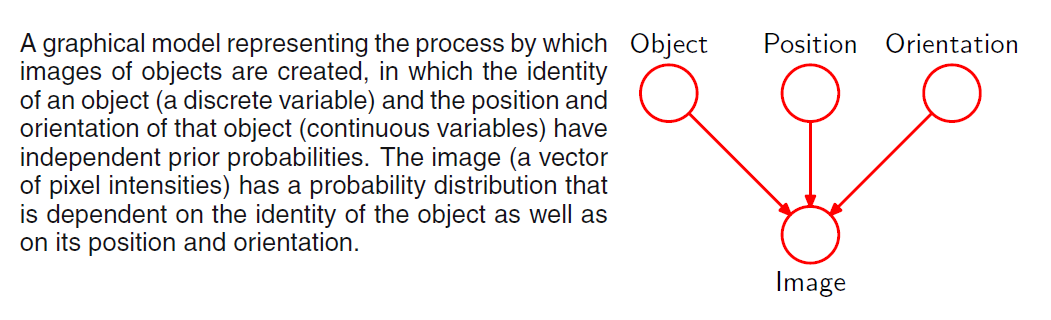Given object, position, orientation, we can sample from the conditional distribution of image and generate pixels.

The graphical model captures causal process by which the observed data was generated. For this reason, such models are often called generative models.

Independence in Bayesian Networks

Our intuition tells us that the parents of a variable “shield” it from probabilistic influence that is causal in nature. In other words, once I know the value of the parents, no information relating directly or indirectly to its parents or other ancestors can influence my beliefs about it. However, information about its descendants can change my beliefs about it, via an evidential reasoning process.

Bayesian Network Semantics

Definition 3.1: Bayesian Network Structure

A Bayesian network structure \(G\) is a directed acyclic graph whose nodes represent random variables \(X_1, ...., X_n\). Let \(Pa^{G}_{X_i}\) denote the parents of \(X_i\) in \(G\), and \(\text{NonDescendants}_{X_i}\) denote the variables in the graph that are not descendants of \(X_i\). Then \(G\) encodes the following set of conditional independence assumptions, called local independence, and denoted by \(I_l (G)\):

\[I_l (G) = \{\text{For each variable $X_i$: ($X_i \perp \text{NonDescendants}_{X_i} | Pa^G_{X_i}$})\}\]

In other words, the local independence state that each node \(X_i\) is conditionally independent of its non-descendants given its parents.

Graphs and Distributions

We now show that the previous two definitions of BN are equivalent. That is, a distribution \(P\) satisfies the local independence associated with a graph \(G\) IFF \(P\) is representable as a set of CPDs associated with the graph \(G\).

I-Maps

Definition 3.2: Independencies in \(P\)

Let \(P\) be a distribution over \(\mathbf{X}\). We define \(I(P)\) to be the set of independence assertions of the form \((\mathbf{X} \perp \mathbf{Y} | \mathbf{Z})\)

Definition 3.3: I-Map

Let \(K\) be any graph object associated with a set of independencies \(I(K)\). We say that \(K\) is an I-map for a set of independencies \(I\) if \(I(K) \subseteq I\).

We now say that \(G\) is a I-map for \(P\) if \(G\) is an I-map for \(I(P)\). That is \(I(G) \subseteq I(P)\).

That is, for \(G\) to be an I-map of \(P\), it is necessary that \(G\) does not mis-lead us regarding independencies in \(P\): any dependence that \(G\) asserts must also hold in \(P\). Conversely, \(P\) may have additional independencies that are not reflected in \(G\).

I-Map to Factorization

A BN structure \(G\) encodes a set of conditional independence assumptions, every distribution for which \(G\) is an I-map must satisfy these assumptions.

Definition 3.4: Factorization (Chain Rule of Bayesian Network)

Let \(G\) be a BN graph over the variables \(X_1, ...., X_n\). We say that a distribution \(P\) over the same space factorizes according to \(G\) if \(P\) can be expressed as a product:

\[P(X_1, ...., X_n) = \prod^n_{i=1} P(X_i | Pa^G_{X_i})\]

Definition 3.5: Bayesian Network

A Bayesian network is a pair \(B = (G, P)\) where \(P\) factorizes over \(G\), and where \(P\) is specified as a set of CPDs associated with \(G\)'s nodes. The distribution \(P\) is often annotated \(P_B\).

Theorem 3.1: I-Map Factorization

Let \(G\) be a BN structure over a set of random variables \(\mathbb{X}\), and let \(P\) be a joint distribution over the same space. If \(G\) is a I-map for \(P\), then \(P\) factorizes according to \(G\) (can be written in the form as in definition 3.4).

Factorization to I-Map

Theorem 3.2: Factorization to I-Map

Let \(G\) be a BN structure over a set of random variables \(\mathbb{X}\) and let \(P\) be a joint distribution over the same space. If \(P\) factorizes according to \(G\), then \(G\) is an I-map for \(P\).

Independencies in Graphs

Knowing only that a distribution \(P\) factorizes over \(G\), we can conclude that it satisfies \(I_l (G)\). Are there other independencies that hold for every distribution \(P\) that factorizes over \(G\)? Our goal is to understand when we can guarantee that an independence \((\mathbf{X} \perp \mathbf{Y} | \mathbf{Z})\) holds in a distribution associated with a BN structure \(G\).

D-Separation

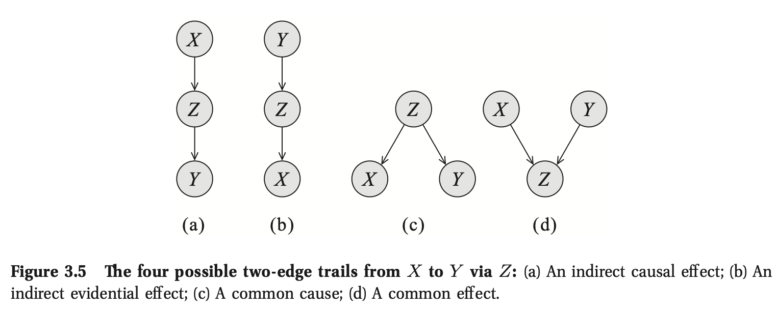
When influence can flow from \(X, Y\) via \(Z\) (\(X, Y\) are correlated), we say that the trail is active

• Direct connection: When \(X, Y\) are directly connected via edge. For any network structure \(G\) they are always correlated regardless of any evidence about any of the other variables in the network.
• Indirect connection: \(X, Y\) are not directly connected via edge, but there is a trail between then in the graph via \(Z\).
  • Indirect causal effect: \(X \rightarrow Z \rightarrow Y\). If we observe \(Z\), then \(X, Y\) are conditionally independent, if \(Z\) is not observed, \(X\) influences \(Y\) by first sampling from \(P(X)\) then sampling \(Z\) from \(P(Z | X)\), so \(X, Y\) are not independent. (Active IFF \(Z\) is not observed)
  • Indirect evidential effect: \(Y \rightarrow Z \rightarrow X\), same as indirect causal effect. (Active IFF \(Z\) is not observed)
  • Common cause: \(X \leftarrow Z \rightarrow Y\), same as above, \(X\) can influence \(Y\) via \(Z\) IFF \(Z\) is not observed. (Active IFF \(Z\) is not observed)
  • Common effect: \(X \rightarrow Z \leftarrow Y\), if \(Z\) is unobserved, then \(X, Y\) are independent, if it is observed then they are not. (Active IFF \(Z\) or one of \(Z\)'s descendants is observed)

Definition 3.6: General Case (One path from \(X_1\) to \(X_n\))

Let \(G\) be a BN structure, and \(X_1 \rightleftharpoons .... \rightleftharpoons X_n\) a trail in \(G\). Let \(\mathbf{Z}\) be a subset of observed variables. The trail \(X_1 \rightleftharpoons .... \rightleftharpoons X_n\) is active given \(\mathbf{Z}\) if:

• Whenever we have a \(v\)-structure (Common effect), then \(X_i\) or one of its descendants are in \(\mathbf{Z}\).
• No other node along the trail is in \(\mathbf{Z}\).

Note if \(X_1\) or \(X_n\) are in \(\mathbf{Z}\), the trail is not active.

Definition 3.7: D-seperation

Let \(\mathbf{X}, \mathbf{Y}, \mathbf{Z}\) be three sets of nodes in \(G\). We say that \(\mathbf{X}, \mathbf{Y}\) are d-seperated given \(\mathbf{Z}\), denoted \(d-sep_G(\mathbf{X}; \mathbf{Y} | \mathbf{Z})\), if there is no active trail between any node \(X \in \mathbf{Z}\) and \(Y \in \mathbf{Y}\) given \(\mathbf{Z}\). We use \(I(G)\) to denote the set of independencies that correspond to d-separation:

\[I(G) = \{(\mathbf{X} \perp \mathbf{Y} | \mathbf{Z}) : d-sep_{G} (\mathbf{X}; \mathbf{Y} | \mathbf{Z})\}\]

The independencies in \(I(G)\) are precisely those that are guaranteed to hold for every distribution over \(G\).

Soundness and Completeness

Theorem 3.3: Soundness

If a distribution \(P\) factorizes according to \(G\), then \(I(G) \subseteq I(P)\).

In other words, any independence reported by d-separation is satisfied by the underlying distribution.

Definition 3.8: Faithful

A distribution \(P\) is faithful to \(G\) if, whenever \((X \perp Y | \mathbf{Z}) \in I(P)\), then \(d-sep_G(X; Y | \mathbf{Z})\).

In other words, any independence in \(P\) is reflected in the d-separation properties of the graph.

Theorem 3.4: Completeness

Let \(G\) be a BN structure. If \(X, Y\) are not d-separated given \(\mathbf{Z}\) in \(G\), then \(X, Y\) are dependent given \(\mathbf{Z}\) in some distribution \(P\) that factorizes over \(G\).

THese results state that for almost all parameterizations \(P\) of the graph \(G\), the d-separation test precisely characterizes the independencies that hold for \(P\).

Conditional Independence

An important concept for probability distributions over multiple variables is that of conditional independence. Consider three random variables \(A, B, C\) and suppose that the conditional distribution of \(A\), given \(B, C\) is such that it does not depend on the value of \(B\), so that:

\[P(A | B, C) = P(A | C)\]

Then:

\[P(A, B | C) = P(A | B, C) P(B | C) = P(A | C) P (B | C)\]

Thus, we can see that \(A, B\) are statistically independent given \(C, \; \forall C\). Note that this definition of conditional independence will require the above equation holds for all values fo \(C\) and not just for some values. The shorthand notation for conditional independence is:

\[A \perp \!\!\! \perp B \;|\; C\]

An important and elegant feature of graphical models is that conditional independence properties of the joint distribution can be read directly from the graph without having to perform any analytical manipulations. The general framework for achieving this is called d-seperation (d stands for directed).

Three example graphs

We start by illustrating the key concepts of d-separation by three motivating examples.

1. \(P(A, B, C) = P(A | C) P(B | C) P(C)\) 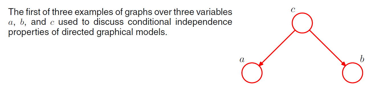\(A, B\) are generally not statistically independent. However, we can easily see that \(A, B\) are conditionally independent given \(C\): \[P(A, B | C) = \frac{P(A, B, C)}{P(C)} = P(A | C) P (B | C)\]

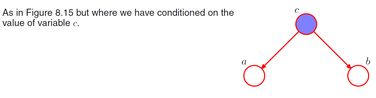
We can provide a simple graphical interpretation of this result by considering the path from node \(A\) to node \(B\) via \(C\). The node \(C\) is said to be tail-to-tail with respect to this path because the node is connected to the tails of the two arrows. However, when we condition on node \(C\) (observed \(C\)), the conditional node blocks the path from \(A\) to \(B\) so causes then to become conditionally independent.

2. \(P(A, B, C) = P(B | C) P(C | A) P (A)\) 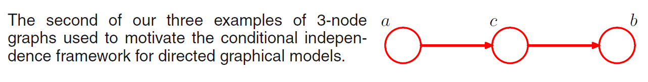\(A, B\) are generally not statistically independent. However, we can easily see that \(A, B\) are conditionally independent given \(C\) by: \[P(A, B | C) = \frac{P(A, B, C)}{P(C)} = P(A | C) P (B | C)\]

We can provide a simple graphical interpretation of this result by considering the path from node \(A\) to node \(B\) via \(C\). The node \(C\) is said to be head-to-tail with respect to this path because the node is connected to the head and tail of the two arrows. However, when we condition on node \(C\) (observed \(C\)), the conditional node blocks the path from \(A\) to \(B\) so causes then to become conditionally independent.

3. \(P(A, B, C) = P(A)P(B)P(C | A, B)\) 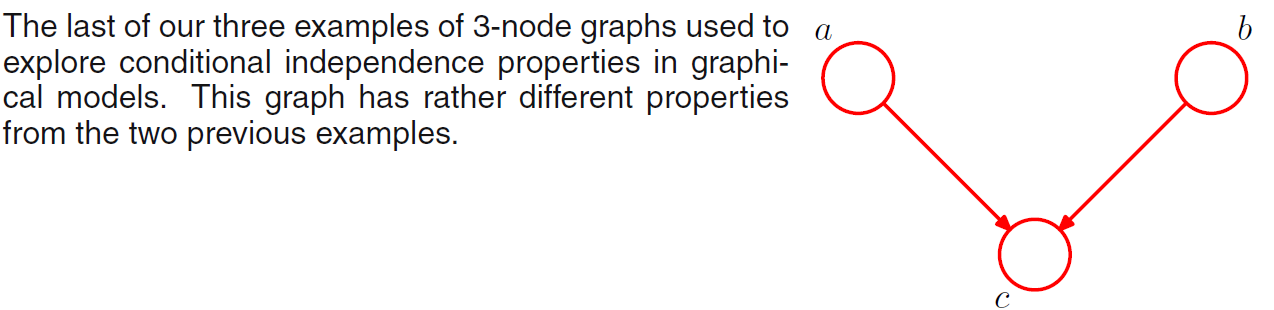We can easily see that \(A, B\) are not conditionally independent. However, we can see that \(A, B\) are statistically independent: \(P(A, B) = \sum_{C} P(A)P(B)P(C | A, B) = P(A)P(B)\)

Thus, our third example has the opposite behaviour from the first two. The node \(C\) is said to be head-to-head with respect to this path because the node is connected to the heads of the two arrows. When the node \(C\) is not given (unobserved), it blocks the path so \(A\) and \(B\) is independent, however, when the node \(C\) is given, \(A\) and \(B\) becomes dependent.

There is one more relationship associate with third example. First we say that node \(Y\) is a descendant of node \(X\) if there is a path from \(X\) to \(Y\) in which each step of the path follows the directions of the arrows. Then it can be shown that a head to head path will become unblocked if either the node or any of its descendants is observed.

D-separation

Consider a general directed graph in which \(A, B, C\) are arbitrary sets of nodes. We wish to ascertain whether a particular conditional independence statement \(A \perp \!\!\! \perp B \;|\; C\) is implied by a given directed acyclic graph. To do so, we consider all possible paths from any node in \(A\) to any node in \(B\). Any such path is said to be blocked if it includes a node such that either:

1. The arrows on the path meet either head-to-tail or tail-to-tail at the node, and the node is in the set \(C\).
2. The arrows meet head-to-head at the node, and neither the node, nor any of its descendants, is in the set \(C\).

If all paths are blocked, then \(A\) is said to be d-separated from \(B\) by \(C\), and the joint distribution over all of the variables in the graph will satisfy \(A \perp \!\!\! \perp B \;|\; C\).

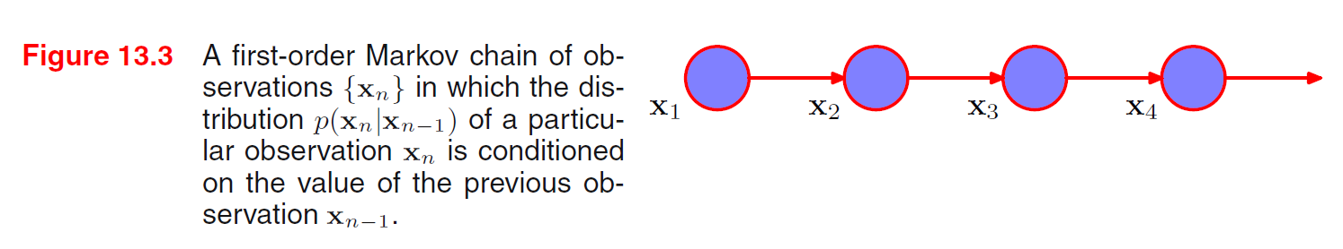
Consider the problem of finding the posterior distribution for the mean of an univariate Gaussian distribution. This can be represented by the directed graph in which the joint distribution is defined by a prior \(P(\mu)\) and \(P(\mathbf{X} | \mu)\) to form the posterior distribution: \[P(\mu | \mathbf{X}) = P(\mu) P(\mathbf{X} | \mu) \] 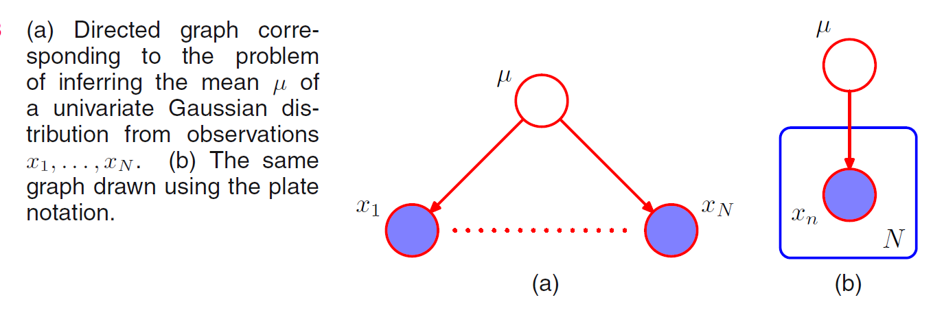In practice, we observe \(D = \{X_1, ...., X_N\}\) with conditional distribution \(P(X_1 | \mu) , ...., P(X_N | \mu)\) respectively, and our goal is to infer \(\mu\). Using d-separation, we note that there is a unique path from any \(X_i\) to any other \(X_{j\neq i}\) and that this path is tail-to-tail with respect to the observed node \(\mu\). Every such path is blocked and so the observations \(D=\{X_1, ..., X_N\}\) are independent given \(\mu\): \[P(\mathbf{X} | \mu) = \prod^N_{i=1} P(X_i | \mu)\] However, if we do not conditional on \(\mu\), the data samples are not independent: \[P(\mathbf{X}) = \int_{\mu} P(\mathbf{X} | \mu) P(\mu) \neq \prod^N_{i=1} P(X_i)\]

Markov Random Fields

Directed Graphical models specify a factorization of the joint distribution over a set of variables into a product of local conditional distributions. They also defined a set of conditional independence properties that must be satisfied by any distribution that factorizes according to the graph. A Markove random field has:

1. A set of nodes each of which corresponds to a random variable or group of random variables
2. A set of links each of which connects a pair of nodes. The links are undirected that is they do not carry arrows.

Conditional Independence Properties

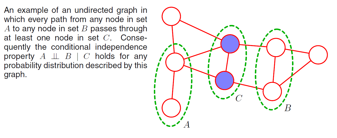
Testing for conditional independence in undirected graph is simpler than in directed graph. Let \(A, B, C\) be three sets of nodes and we consider the conditional independence property \(A \perp \!\!\! \perp B \;|\; C\). To test whether this property is satisfied by a probability distribution defined by the graph:

• Consider all possible paths that connect nodes in set \(A\) to nodes in set \(B\). If all such paths pass through one or more nodes in set \(C\), then all such paths are blocked and so the conditional independence properties holds. If there is at least one such path that is not blocked, then there will exist at least some distributions corresponding to the graph that do not satisfy this conditional independence relation.

Factorization Properties

We now express the joint distribution \(P(\mathbf{X})\) as a product of functions defined over set of random variables that are local to the graph.

If we consider two nodes \(X_i\) and \(X_j\) that are not connected by a link, then these variables must be conditionally independent given all other nodes in the graph, because there is no direct path between the two nodes and all other paths are blocked:

\[P(X_i, X_j | \mathbf{X}_{k\notin \{i, j\}}) = P(X_i | \mathbf{X}_{k\notin \{i, j\}}) P(X_j | \mathbf{X}_{k\notin \{i, j\}})\]

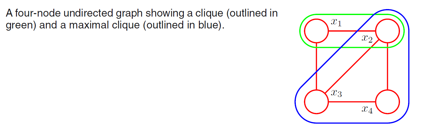
A clique is a subset of nodes in a graph such that there exists a link between all pairs of nodes in the subset. In other words, the nodes in the set are fully connected. Furthermore, a maximal clique is a clique such that it is not possible to include any other nodes from the graph in the set without it ceasing to be a clique.

We can therefore define the factors in the decomposition of the joint distribution to be functions of the variables in the cliques. In fact, we can consider functions of the maximal cliques, without loss of generality because other cliques must be subsets of maximal cliques.

Let \(C\) be a clique and the set of random variables in that clique by \(\mathbf{X}_C\). Then the joint distribution is written as a product of potential functions \(\psi_C(\mathbf{x}_C) \geq 0\) over the maximal cliques of the graph:

\[P(\mathbf{X}) = \frac{1}{Z} \prod_{C} \psi_{C} (\mathbf{X}_C)\]

Here the quantity \(Z\) is called partition function which is used for normalization to ensure the result is a proper joint distribution:

\[Z = \sum_{X} \prod_{C} \psi_{C} (\mathbf{X}_C)\]

In directed graph, we have the links to be conditional distribution, in undirected graph, we do not restrict the choice of potential functions.

Ref

PRML chapter 8

LightGBM: A Highly Efficient Gradient Boosting Decision Tree

Background

GBDT

GBDT is an ensemble model of decision trees, which are trained in sequence. In each iteration, GBDT learns the decision trees by fitting the negative gradients (also known as residual errors).

The main cost in GBDT lies:

1. Learning the decision trees (finding the best split points) when there is large number of features and samples.
   • Histogram based algorithm buckets continuous feature values into discrete bins and uses these bins to construct feature histograms during training. It finds the best split points based on the feature histogram, the criterion is calculated at the interval boundaries. It costs \(O(N \times M)\) for histogram building and \(O(\text{Number of bins} \times M)\) for split point finding. Since number of bins is much smaller than number of data points, histogram building will dominate the computational complexity.
   • Pre-sorted algorithm sorts the values of each numeric attribute, and evaluates the criterion at each possible split point to find the splitting point with the minimum criterion. The sorting requires \(O(n\log (n))\).
2. Number of Samples:
   • Down sampling the data instance (i.e weights, random subsets), most of the algorithms are based on adaboost which has weights but not GBDT which does not have weights natively. Random subsets hurt the performance.
3. Number of Features:
   • PCA to remove weak correlated features (depends on assumption that features contain significant redundancy which might not always be true in practice)

Gradient-based One-Side Sampling

In AdaBoost, the sample weight serves as a good indicator for the importance of data instances. In GBDT, gradient for each data instance provides us with useful information for data sampling. That is, if an instance is associated with a small gradient, the training error for this instance is small and it is already well-trained. A straightforward idea is to discard those data instances with small gradients. However, the data distribution will be changed by doing so. To avoid this problem, GOSS keeps all the instances with large gradients and performs random sampling on the instances with samll gradients.

In order to compensate the influence to the data distribution, when computing the information gain, GOSS introduces a constant multiplier for the data instances with samll gradients. Specifically, GOSS:

1. Firstly sorts the data instances according to the absolute value of their gradients.
2. Selects the top \(a \times 100%\) instances.
3. Then it randomly samples \(b \times 100%\) from the rest of the data.
4. Amplifies the sampled data with small gradients by a constant \(\frac{1 - a}{b}\) when calculating the criterion to normalize the sum of the gradients.

Exclusive Feature Bundling

High-dimensional data are usually very sparse. The sparsity of the feature space provides us a possibility of designing a nearly lossless approach to reduce the number of features. Specifically, in a sparse feature space, many features are mutually exclusive (they never take nonzero values simultaneously), we can safely bundle these features into a single feature. In this way, the complexity of histogram building changes from \(O(N \times M)\) to \(O(N \times \text{Number of bundles})\). Then we can significantly speed up the training of GBDT without hurting the accuracy.

Which Features to Bundle

Partitioning features into smallest number of exclusive bundles is NP-hard, thus it is impossible to find an exact solution within polynomial time. Thus, a greedy algorithm which can produce reasonable good results are being used. Furthermore, we can allow a small fraction of conflicts which is controlled by \(\gamma\) (there are usually quite a few features, although not 100% mutually exclusive, also rarely take nonzero values simultaneously) to have an even smaller number of feature bundles and further improve the computational efficiency. For small \(\gamma\), we will be able to achieve a good balance between accuracy and efficiency.

Intuitively, it:

1. Builds a graph with features as vertices and weighted edges as total conflicts between features (Edge only occurs when two features are not mutually exclusive).
2. Sort the features by their degrees (Number of edges)
3. Check each feature in the ordered list and either append it to existing list (if total conflicts between feature and bundle less than \(\gamma\)) or create a new bundle.

The time complexity of algorithm 3 is \(O(M^2)\) and it is only processed once before training. This complexity is acceptable when the number of features is not very large.

How to Construct the Bundle

The key is to ensure that the values of the original features can be identified from the feature bundles. This can be done by adding offsets to the original values of the features:

1. Calculate the offset to be added to every feature in feature bundle.
2. Iterate over every data instance and feature.
3. Initialize the new bucket as zero for instances where all features are zero.
4. Calculate the new bucket for every non zero instance of a feature by adding respective offset to original bucket of that feature

Ref

https://www.researchgate.net/publication/351133481_Comparison_of_Gradient_Boosting_Decision_Tree_Algorithms_for_CPU_Performance

https://papers.nips.cc/paper/2017/file/6449f44a102fde848669bdd9eb6b76fa-Paper.pdf

https://robotenique.github.io/posts/gbm-histogram/

https://www.aaai.org/Papers/KDD/1998/KDD98-001.pdf

ROC Curve

ROC Curve is a graph showing the performance of a classification model at all classification thresholds (e.g for logistic regression the threshold is default 0.5, we can adjust this threshold to 0.8 and assign examples to classes using this threhold). This curve plots two parameters:

• True Positive Rate (\(\text{sensitivity} = \frac{\text{True Positive}}{\text{True Positive + False Negative}}\))
• False Positive Rate (\(1 - \text{specificity} = 1 -\frac{\text{True Negative}}{\text{True Negative + False Positive}} = \frac{\text{False Positive}}{\text{True Negative + False Positive}}\))

An ROC curve plots TRP vs FPR at different classification thresholds. Lowering the classification threshold classifies more items as positive (e.g threshold 0.1 for logistic regression), thus increasing both FP and TP.

To compute the points an ROC curve, we could evaluate a classification model many times with different threshold and repeat this for all thresholds, but this is inefficient. Fortunately, there's an effective algorithm that can provide this information called AUC.

AUC

AUC stands for Area under ROC curve. It measures the entire two-dimensional area underneath the entire ROC curve. Since \(TPR \in [0, 1]\) and \(FPR \in [0, 1]\), the AUC can be interpreted as probability. It is the probability that the model ranks a random positive example more highly than a random negative example. Thus, by rearranging the predictions from left to right, AUC is the probability that a random positive example is positioned to the right of a random negative example:

A model whose predictions are 100% wrong will have AUC 0, a model whose predictions are 100% correct has an AUC of 1.

Properties

AUC is desirable for the following two reasons:

• Scale-invariant: It measures hwo well predictions are ranked, rather than their absolute values.
• Classification-threshold-invariant: It measures the quality of the model's predictions irrespective of what classification threshold is chosen. (when we draw ROC, we are varying the threshold, the only thing matters to AUC is the predicted values (not class) and how true positive class samples ranked against negative class samples w.r.t their predicted values)

However, AUC is not desirable when:

1. Sometimes probabilities matters, AUC does not tell you how good is a predicted probability.
2. Sometimes classification threshold matters, In cases where there are wide disparities in the cost of false negatives vs. false positives, it may be critical to minimize one type of classification error. For example, when doing email spam detection, you likely want to prioritize minimizing false positives (even if that results in a significant increase of false negatives). AUC isn't a useful metric for this type of optimization.

Ref

https://developers.google.com/machine-learning/crash-course/classification/roc-and-auc

Neural Machine Translation By Jointly Learning to Align and Translate

One problem with traditional encoder-decoder structure is that a neural network needs to be able to compress all the necessary information of a source sentence into a fixed-length vector \(\mathbf{c}\). Attention does not attempt to encode a whole input sentence into a single fixed-length vector. Instead, it encodes the input sentence into a sequence of vectors and chooses a subset of these vectors adaptively while decoding the translation.

Background: RNN Encoder-Decoder

In the Encoder-Decoder framework, an encoder reads the input sentence, a sequence of vectors \(\mathbf{x} = (\mathbf{x}_1, ...., \mathbf{x}_{T_x})\), into a fixed length context vector \(\mathbf{c}\):

\[\mathbf{h}_t = f(\mathbf{x}_t, \mathbf{h}_{t-1})\] \[\mathbf{c} = q(\mathbf{h}_{1}, ...., \mathbf{h}_{T_x})\]

Where \(f\) and \(q\) are non-linear functions. Typically, \(q\) is the identity function defined as \(q(\mathbf{h}_{1}, ...., \mathbf{h}_{T_x}) = \mathbf{h}_{T_x}\).

The decoder is often trained to predict the next word \(\mathbf{y}_{t^{\prime}}\) given all the previous predicted words \(\{\hat{\mathbf{y}}_1, ..., \hat{\mathbf{y}}_{t^{\prime} - 1}\}\). In training step \(t\), we can use feed the true target value \(\mathbf{y}_{t-1}\). Then, in training of decoder, we are maximizing the log joint conditional probability (minimize the sum of per time step cross entropy):

\[L = \sum^{T_y}_{t=1} L^{t}\] \[-L = P_{\mathbf{Y}}(\mathbf{y}) = \sum^{T_y}_{t=1} P_{\mathbf{Y_t} | \mathbf{Y_1} ,...., \mathbf{Y_{t-1}}, \mathbf{c}}(\mathbf{y}_t | \{\mathbf{y}_{1}, ...., \mathbf{y}_{t-1}, \mathbf{c}\})\]

Where in RNN, each conditional probability distribution \(P_{\mathbf{Y_t} | \mathbf{Y_1} ,...., \mathbf{Y_{t-1}}, \mathbf{c}}\) is model as \(g(\mathbf{y}_{t-1}, \mathbf{s}_t, \mathbf{c})\).

Learning to Align and Translate

Attention contains bidirectional RNN as an encoder and a decoder that emulates searching through a source sentence during decoding a tranlation.

Decoder: General Description

In the new model, we define each conditional distribution as:

\[\hat{P}_{\mathbf{Y_t} | \mathbf{Y_1} ,...., \mathbf{Y_{t-1}}, \mathbf{c}} \triangleq g(\mathbf{y}_{t-1}, \mathbf{s}_t, \mathbf{c}_t)\]

Notice here, we have different \(\mathbf{c}_t\) for each time step \(t\).

The context vector \(\mathbf{c}_i\) depends on a sequence of annotations \((\mathbf{h}_1, ....., \mathbf{h}_{T_x})\) which contains information about the whole input sequence (similar to hidden units in encoder) with a strong focus on the parts surrounding the \(i\)th word of the input sequence.

The context vector \(\mathbf{c}_i\) is, then computed as a weighted sum of these annotations \(\mathbf{h}_{i}\):

\[\mathbf{c}_i = \sum^{T_x}_{j=1} \alpha_{ij} \mathbf{h}_j\]

\[\alpha_{ij} = \frac{\exp^{e_{ij}}}{\sum^{T_x}_{k=1} \exp^{e_{ik}}}\]

Where

\[e_{ij} = a(\mathbf{s}_{i-1}, \mathbf{h}_j)\]

is an alignment model which scores how well the inputs around position \(j\) and the output at position \(i\) match. This model \(a\) is parameterized by a MLP which is jointly trained with all the other components of the proposed system. The score is based on the RNN decoder's hidden state \(\mathbf{s}_{i-1}\) and the \(j\)th annotation \(\mathbf{h}_j\) of the input sentence. It reflects the importance of each annotation vector \(\mathbf{h}_j\) with respect to the previous hidden state \(\mathbf{s}_{i-1}\) in deciding the current state \(\mathbf{s}_i\) and generating prediction \(\hat{\mathbf{y}}_i\).

We can think the approach of taking a weighted sum of all the annotations as computing an expected annotation, where the expectation is over possible alignments (\(\alpha_{ij}\)). In other words, let \(\alpha_{ij}\) be a probability that the target word \(\mathbf{y}_i\) is aligned to, or translated from a source input word \(\mathbf{x}_{j}\). Then, the \(i\)th context vector \(\mathbf{c}_i\) is the expected value of annotations (input sequence) distributed according to probability distribution defined by \(\alpha_{ij}\).

Intuitively, this implements a mechanism of attention in the decoder. The decoder decides parts of the source sentence to pay attention to. By letting the decoder have an attention mechanism, we relieve the encoder from the burden of having to encode all information in the source sentence into a fixed length vector.

Encoder: Bidirectional RNN for Annotating Sequences

A bidirectional RNN consists of forward and backward RNNs. The forward RNN \(\overset{\rightarrow}{f}\) reads the input sequence from the front and has forward hidden units \(\{\overset{\rightarrow}{\mathbf{h}}_1, ...., \overset{\rightarrow}{\mathbf{h}}_{T_x}\}\). \(\overset{\leftarrow}{f}\) reads the sequence in the reverse order (from \(\mathbf{x}_{T_x}\) to \(\mathbf{x}_1\)), resulting in a sequence of backward hidden units \(\{\overset{\leftarrow}{\mathbf{h}}_1, ...., \overset{\leftarrow}{\mathbf{h}}_{T_x}\}\).

The annotation vector \(\mathbf{h}_j\) is then calculated by concatenating the forward hidden state \(\overset{\rightarrow}{\mathbf{h}}_j\) and the backward hidden state \(\overset{\leftarrow}{\mathbf{h}}_j\):

\[\mathbf{h}_j = [\overset{\rightarrow}{\mathbf{h}}_j, \overset{\leftarrow}{\mathbf{h}}_j]\]

This sequence of annotations is used by the decoder and the alignment model later to compute the context vector \(\mathbf{c}_{i}\).

Effective Approaches to Attention-based Neural Machine Translation

Long Short-Term Memory-Networks for Machine Reading

Ref

https://lilianweng.github.io/lil-log/2018/06/24/attention-attention.html#self-attention

Recurrent Neural Network

Introduction

Consider the recurrent equation:

\[\mathbf{s}^{t} = f(\mathbf{s}^{t-1}; \; \boldsymbol{\theta})\]

For a finite time step \(\tau\), this equation can be unfolded by applying the definition \(\tau - 1\) times:

\[f(f(....f(\mathbf{s}^{1}; \; \boldsymbol{\theta}) ... ; \; \boldsymbol{\theta}) ; \; \boldsymbol{\theta})\]

Then, this expression can now be represented as a DAG because it no longer involves recurrence:

Notice here, the parameters \(\boldsymbol{\theta}\) are shared. The idea extends smoothly to:

\[\mathbf{s}^{t} = f(\mathbf{s}^{t-1}, \mathbf{x}^{t}; \; \boldsymbol{\theta})\]

We can see that now, \(s^{t}\) contains information about the whole past \(\mathbf{x}^1 , ....., \mathbf{x}^t\)

Many Recurrent Neural Networks use similar idea to express their hidden units:

\[\begin{aligned} \mathbf{h}^t &= f(\mathbf{h}^{t-1}, \mathbf{x}^t ; \; \boldsymbol{\theta})\\ &= g^t (\mathbf{x}^1 , ....., \mathbf{x}^t) \end{aligned}\]

Typically, RNN will have output layers to output predictions at given timesteps. When the recurrent network is trained to perform a task that requires predicting the future from the past, the network typically learns to use \(\mathbf{h}^t\) to give a lossy summary of past sequence up to time \(t\). The summary is lossy because we are mapping \(\mathbf{x}^1 , ....., \mathbf{x}^t\) to a fixed length \(\mathbf{h}^t\)

The unfolded structure has several advantages:

1. The learned model \(f\) is defined as transition from hidden units (input) \(h^{t - 1}\) to \(h^{t}\) (output) regardless the value of time \(t\). Thus, we can have one model for different lengths of sequences.
2. The parameters \(\boldsymbol{\theta}\) are shared.