ADAM: A METHOD FOR STOCHASTIC OPTIMIZATION

Let \(F\) be a noisy objective function (stochastic function) defined as \(F(\boldsymbol{\theta})\) that is differentiable w.r.t \(\boldsymbol{\theta}\), we are interested in minimizing the expected value of this random function:

\[\min_{\boldsymbol{\theta}} E_{F}[F(\boldsymbol{\theta})]\]

Let \(F_1(\boldsymbol{\theta}), ...., F_{T} (\boldsymbol{\theta})\) be a random sample of \(F(\boldsymbol{\theta})\) and let \(f_1 (\boldsymbol{\theta}), ..., f_T(\boldsymbol{\theta})\) be the realization of random sample. This random sample can be forms of mini-batches of data which the distribution does not depend on the parameter \(\boldsymbol{\theta}\).

Then:

\[\nabla_{\boldsymbol{\theta}} E_F[F (\boldsymbol{\theta})] = E_F[\nabla_{\boldsymbol{\theta}} F (\boldsymbol{\theta})]\]

Given the individual sample gradient \(\nabla_{\boldsymbol{\theta}} f_1 (\boldsymbol{\theta}), ...., \nabla_{\boldsymbol{\theta}} f_T(\boldsymbol{\theta})\), one way to estimate the expectation of gradient, \(E_{F} [\nabla_{\boldsymbol{\theta}} F_t(\boldsymbol{\theta})]\), is to use stochastic approximation (similar to Momentum):

\[m_t \leftarrow \beta_1 {m}_{t} + (1 - \beta_1) \nabla_{\boldsymbol{\theta}} f_t(\boldsymbol{\theta})\]

Where \(m_t\) is the average up to sample \(t\), and \(\beta_1 \in [0, 1)\) is the decay rates.

At the same time, we can use SA to estimate the second moment of the gradient which is the un-centered variance (This is similar to RMSProp):

\[v_t \leftarrow \beta_2 {v}_{t} + (1 - \beta_2) \nabla_{\boldsymbol{\theta}} f_t(\boldsymbol{\theta})^2\]

However, these estimates are biased toward 0 if we initialize them to be 0 especially during initial timesteps and especially when the decay rates are small (\(\beta_1, \beta_2\) close to 1). Thus, we need to apply bias correction.

Initial Bias Correction

Let \(\mathbf{G} = \nabla_{\boldsymbol{\theta}} F\) be the gradient of the stochastic objective \(F\), we wish to estimate its second raw moment using SA of the squared gradient with decay rate \(\beta_2\). Let \(\mathbf{G}_1, ...., \mathbf{G}_T\) be random sample of \(\mathbf{G}\) that draws from the gradient distribution \(P(\mathbf{G})\). Suppose we initialize our SA procedure at \({v}_0 = 0\), then after \(t\) steps, we have:

\[v_1 = (1 - \beta_2) \mathbf{G}^2_1\]

\[v_2 = \beta_2(1 - \beta_2) \mathbf{G}^2_1 + (1 - \beta_2) \cdot \mathbf{G}^2_2 = \beta_2 (1 - \beta_2) (\mathbf{G}^2_1 + \mathbf{G}^2_2)\]

\[\implies {v}_t = (1 - \beta_2) \sum^{t}_{i=1} \beta^{t - i}_2 \mathbf{G}^2_{i}\]

Where \(\mathbf{G}^2 = \|\mathbf{G}\|^2_2\). We want the SA estimator to be unbiased estimator of second moment of gradient but we know that there is initialization bias (discrepancy) of SA estimator, we denote this discrepancy \(\eta\). Since additive discrepancy can be keep small by assigning less weight to history, we want two sides to be equal:

\[E_{\mathbf{G}} [\mathbf{G}^2] = E_\mathbf{G}[\mathbf{v}^2_t] + \eta = E_\mathbf{G} [(1 - \beta_2) \sum^{t}_{i=1} \beta_2^{t - i} \mathbf{G}^2_{i}] + \eta\]

However, since \(t < \infty\), we have a proportion bias:

Thus, we can apply a bias correction term on the estimator to correct for this proportion bias \(\frac{1}{1 - \beta^t_2}\).

The same correction \(\frac{1}{1 - \beta^t_1}\)is applied on first moment estimator of the gradient.

AdaMax

In Adam, the current average gradient estimate \(\hat{m}_t\) is scaled inversely to history proportional to the scaled \(L^2\) norm of their individual current and past gradients (i.e \(\frac{\alpha}{\sqrt{\hat{v}_t} + \epsilon}\)). We can generalize \(L^2\) norm to a \(L^\infty\) norm based update rule. This leads to a surprisingly simple and stable algorithm:

In case of \(L^p\) norm, \(\mathbf{v}_t\) is defined to be:

Note define:

\[u_t = \lim_{p \rightarrow \infty} (v_t)^{\frac{1}{p}}\]

Then:

Which corresponding to:

\[u_t \leftarrow \max(\beta_2 u_{t}, \|\mathbf{G}_t\|_{\infty})\]

Algorithms with Adaptive Learning Rates

Learning rate is reliably one of the hyperparameters that is the most difficult to set because it has a significant impact on model performance. At each iteration, the cost is often highly sensitive to some directions in parameter space and insensitive to others. Momentum solves some of the problems in the cost of introducing another hyperparameter. Thus, it is natural to consider algorithms that have separate learning rate for each parameter and automatically adapt learning rates for each of the parameter.

The delta-bar-delta algorithm (base on full-batch) is an early heuristic approach to adapting individual learning rates for model parameters during training, it is based on intuitive idea similar to momentum:

If the partial derivative of the loss, with respect to a given model parameter, remains the same sign, then the learning rate should increase, if the partial derivative with respect to the parameter changes sign, then the learning rate should decrease.

We would like to extend the idea to mini-batch scenario.

AdaGrad

The AdaGrad algorithm, individually adapts the learning rates of all model parameters by scaling them inversely proportional to square root of the sum of all of their historical squared values:

1. If \(g_1\) is large constantly larger than \(g_2\), then:

   \[\sqrt{r_1} > \sqrt{r_2} \implies \epsilon_1 < \epsilon_2\]

   This makes sense because we want to take a small step in the gradient direction when the magnitude of gradient is large, especially when we have noisy gradient. Conversely, we would like to take slightly larger step than large gradient case when we have smaller gradient.

2. If \(r_i\) is less than 1, we have increasing learning rate compare to base learning rate:

   \[r_i < 1 \implies \epsilon_i > \epsilon\]

   This helps us to get out of the local minimum or flat region of the surface by taking larger steps.

AdaGrad is designed to converge rapidly when applied to a convex optimization problem, so when it finds a convex structure, it can converge rapidly.

However, in non-convex optimization problem (training neural networks) the accumulated gradient \(\mathbf{r}\) starts accumulating at the beginning, this will introduce excessive decrease in the effective learning in later training steps (at end, we will have large \(\mathbf{r}\), so the learning rates will be small to prevent effective learning in later stages or early large gradients will prevent learning in early stages).

RMSProp

The RMSProp algorithm modifies AdaGrad so that it can perform better in non-convex setting by changing the gradient accumulation into an exponentially weighted moving average, so the early accumulation becomes less and less important. This structure helps in non-convex problem by discarding the history from extreme past so when we arrive at a convex bowl, we have sufficiently large learning rate to converge rapidly.

The algorithm introduces a new parameter \(\rho\) that controls for the weight of accumulated gradient.

Momentum

While SGD remains a very popular optimization strategy, learning with it can be slow. The method of momentum is designed to accelerate learning, especially in the face of high curvature (large change of direction of the curve in small amount time), small but consistent gradients (flat surface) or noisy gradients (with high variance). The momentum algorithm accumulates an exponentially decaying moving average of past gradients and continues to move in their direction.

The momentum algorithm introduces several variables:

1. A vector \(\mathbf{v}\) that plays a role of velocity (with direction and speed). The velocity is set to an exponentially decaying average of the negative gradient.
2. A hyparameter \(\alpha \in [0, 1)\) determins how quickly the contributions of previous gradients exponentially decay.

The update rule is given by:

\[\mathbf{v} \leftarrow \alpha \mathbf{v} - \epsilon \nabla_{\boldsymbol{\theta}} (\frac{1}{N} \sum^{N}_{i=1} L(\mathbf{f} (\mathbf{x}_i; \; \boldsymbol{\theta}), \mathbf{y}_i))\]

\[\boldsymbol{\theta} \rightarrow \boldsymbol{\theta} + \mathbf{v}\]

Previously, in SGD, the size of the step was simply the norm of the gradient multiplied by the learning rate:

\[\epsilon \nabla_{\boldsymbol{\theta}} (\frac{1}{N} \sum^{N}_{i=1} L(\mathbf{f} (\mathbf{x}_i; \; \boldsymbol{\theta}), \mathbf{y}_i))\]

Now the size of the step depends on how large and how aligned a sequence of gradients are. The step size is largest when many successive gradients point in exactly the same direction. If the momentum algorithm always observe gradient \(\mathbf{g}\), then it will accelerate in the direction of \(-\mathbf{g}\):

\[\mathbf{v}_1 \leftarrow - \epsilon \mathbf{g}\]

\[\mathbf{v}_2 \leftarrow -\mathbf{g} \epsilon(\alpha + 1)\]

\[\mathbf{v}_N \leftarrow -\mathbf{g} \epsilon \sum^{N-1}_{i=0} \alpha^i\]

\[\implies \|\mathbf{v}_{\infty}\| = \frac{\epsilon \|\mathbf{g}\|}{1 - \alpha}\]

The terminal velocity will have speed \(\frac{\epsilon \|\mathbf{g}\|}{1 - \alpha} \gg \epsilon \|\mathbf{g}\|\). This makes sense because if we receive consistent small gradients, we would like to take larger steps because we are confident we are in the right direction. One the other hand, consistently changing direction gradients (high curvature) would cause the gradient to be small to allow convergence.

Nesterov Momentum

Nesterov Momentum is inspired by Nesterov's accelerated gradient method, the update rules in this case are given by:

\[\mathbf{v} \leftarrow \alpha \mathbf{v} - \epsilon \nabla_{\boldsymbol{\theta}} (\frac{1}{N} \sum^{N}_{i=1} L(\mathbf{f} (\mathbf{x}_i; \; \boldsymbol{\theta} + \alpha \mathbf{v}), \mathbf{y}_i))\]

\[\boldsymbol{\theta} \rightarrow \boldsymbol{\theta} + \mathbf{v}\]

This is similar to momentum, but before taking the gradient, we first take one step forward using previous velocity, then we take the gradient there and adjust velocity accordingly. We can also think of this as attempting to add a correlation factor to the standard method of momentum.

Implementation

1
2
3
4
5
6
7
8
9
10
11
12
13
14
15
16
17
18
19
20
21
22
23
24

class SGD:
    def __init__(self, lr, model_vars):
        self.model_vars = model_vars
        self.lr = lr

    def __call__(self, grad):
        for i, v in enumerate(self.model_vars):
            self.model_vars[i] = v - self.lr * grad[i]

        return self.model_vars

class Momentum:
    def __init__(self, lr, model_vars, alpha=0.9):
        self.lr = lr
        self.model_vars = model_vars
        self.alpha = alpha
        self.v = 0
        
    def __call__(self, grad):
        for i, v in enumerate(self.model_vars):
            self.v = self.v * self.alpha - self.lr * grad[i]
            self.model_vars[i] = self.model_vars[i] + self.v

        return self.model_vars

Ref

Soft Actor-Critic: Off-Policy Maximum Entropy Deep Reinforcement Learning with a Stochastic Actor

Introductions and Notations

Maximum entropy reinforcement learning optimizes policies to maximize both the expected return and the expected entropy of the policy.

Expectation-Maximization Algorithm

Gaussian Mixture distribution can be written as a linear superposition of Gaussians in the form:

\[P(\mathbf{X}) = \sum^K_{k=1} \pi_k N(\mathbf{X} | \boldsymbol{\mu}_k, \boldsymbol{\Sigma}_k)\]

Where \(\pi_k\) is the mixing coefficient for each normal component that satisfies the conditions:

\[0 \leq \pi_k \leq 1\] \[\sum^{K}_{k=1} \pi_k = 1\]

Let us introduce a \(K\)-dimensional binary latent random vector \(\mathbf{Z}\) having a 1-of-\(K\) representation in which a particular element \(Z_k \in \{0, 1\}\) is equal to 1 and all other elements are equal to 0 and \(\sum^{K}_{k=1} Z_k = 1\). We define:

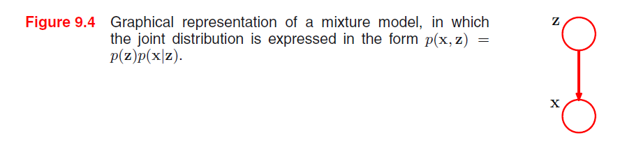
• The joint distribution \(P(\mathbf{X}, \mathbf{Z}) = P(\mathbf{Z}) P(\mathbf{X} | \mathbf{Z})\) in terms of a marginal distribution \(P(\mathbf{Z})\) and a conditional distribution \(P(\mathbf{X} | \mathbf{Z})\).

• The marginal distribution over \(\mathbf{Z}\) is specified in terms of the mixing coefficient \(\pi_k\), such that: \[P(Z_k = 1) = \pi_k\] \[P(\mathbf{Z}) = \prod^{K}_{k=1} \pi_k^{Z_k}\]

• The conditional distribution of \(\mathbf{X}\) given a particular value for \(\mathbf{Z}\) is a Gaussian: \[P(\mathbf{X} | Z_k = 1) = N(\mathbf{X} | \mu_k, \Sigma_k)\] \[P(\mathbf{X} | \mathbf{Z}) = \prod^{K}_{k=1} N(\mathbf{X} | \boldsymbol{\mu}_k, \boldsymbol{\Sigma}_k)^{Z_k}\]

• The conditional probability (posterior probability) of particular value of \(\mathbf{Z}\) given a particular value for \(\mathbf{X}\), which can be found by Bayes rule: \[\gamma(Z_k) = P(Z_k = 1 | \mathbf{X}) = \frac{P(\mathbf{X} | Z_k = 1) P(Z_k = 1)}{P(\mathbf{X})} = \frac{\pi_k N(\mathbf{X} | \boldsymbol{\mu}_k, \boldsymbol{\Sigma}_k)}{\sum^K_{j=1} \pi_k N(\mathbf{X} | \boldsymbol{\mu}_j, \boldsymbol{\Sigma}_j)}\]

  This probability can be viewed as the responsibility that component \(k\) takes for explaining the observation \(\mathbf{X}\)

Then the marginal distribution of the gaussian mixture can be written using the distribution of latent random vector \(\mathbf{Z}\) as:

\[P(\mathbf{X}) = \sum_{\mathbf{Z}} P(\mathbf{Z}) P(\mathbf{X} | \mathbf{Z}) = \sum^{K}_{k=1} \pi_k N(\mathbf{X} | \boldsymbol{\mu}_k, \boldsymbol{\Sigma}_k)\]

It follows that, since we are using a joint distribution, if we have a random sample \(\mathbf{X}_1, ..., \mathbf{X}_N\), for every random vector \(\mathbf{X}_n\) there is a corresponding latent variable \(\mathbf{Z}_n\). Therefore, we have found an equivalent formulation of the Gaussian mixture involving an explicit latent variable. Now, we can work with the joint distribution \(P(\mathbf{X}, \mathbf{Z})\) instead of the original marginal distribution \(P(\mathbf{X})\).

We can express the joint distribution as Bayesian network:

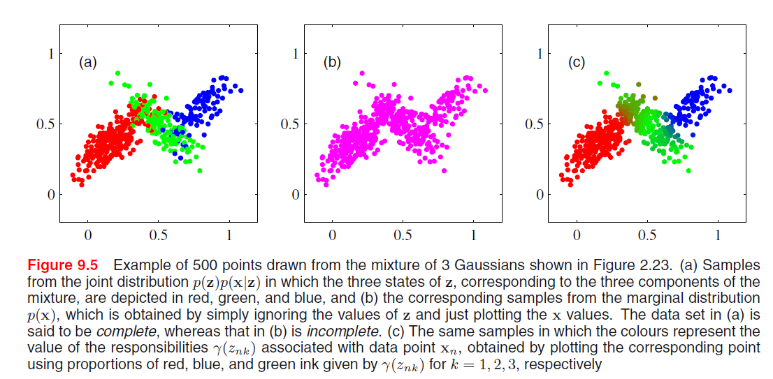
And we can use ancestral sampling to generate random samples distributed according to the Gaussian mixture model:

1. Sample from \(\hat{\mathbf{Z}} \sim P(\mathbf{Z})\)
2. Sample from \(P(\mathbf{X} | \hat{\mathbf{Z}})\)
3. Coloring them by the \(\mathbf{\hat{Z}}\)

EM for Gaussian Mixtures

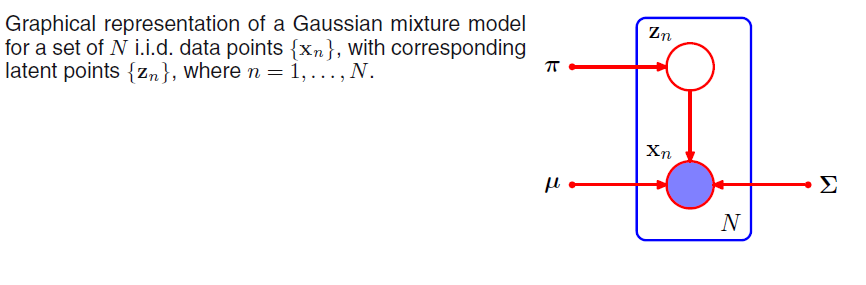
Suppose we have a dataset of observations \(\{\mathbf{x}_1, ...., \mathbf{x}_N; \; \mathbf{x} \in \mathbb{R}^M\}\), and we wish to model this data using a mixture of Gaussians. We can represent this dataset as an \(N \times M\) matrix \(\mathbf{D}\) in which the \(n\)th row is given by \(\mathbf{x}^T_n\). Similarly, the corresponding latent variables will be denoted by an \(N \times K\) matrix \(\mathbf{H}\) with rows \(\mathbf{Z}^T_n\). If we assume that the data points are drawn independently from the distribution then we can express the Gaussian mixture model for this i.i.d dataset using the graphical representation:

The log-likelihood function is given by:

\[\ln(P(\mathbf{D} | \boldsymbol{\pi}, \boldsymbol{\mu}, \boldsymbol{\Sigma})) = \sum^{N}_{n=1} \ln (\sum^K_{k=1} \pi_k N(\mathbf{x}_n | \boldsymbol{\mu}_k, \boldsymbol{\Sigma}_k))\]

An elegant and powerful method for finding maximum likelihood solutions for models with latent variables is called the expectation-maximization algorithm.

We know that at a maximum of the likelihood function (by taking the derivative with respect to \(\mathbf{\mu}_k\)):

\[0 = - \sum^N_{n=1} \underbrace{\frac{\pi_k N(\mathbf{x}_n | \boldsymbol{\mu}_k, \boldsymbol{\Sigma}_k)}{\sum^K_{j=1} \pi_k N(\mathbf{x}_n | \boldsymbol{\mu}_j, \boldsymbol{\Sigma}_j)}}_{\gamma(Z_{nk})} \boldsymbol{\Sigma}_k (\mathbf{x}_n - \boldsymbol{\mu}_k)\]

By assuming that \(\boldsymbol{\Sigma}_k\) is invertible and rearranging we have:

\[\boldsymbol{\hat{\mu}}_k = \frac{1}{N_k} \sum^N_{n=1} \gamma(Z_{nk}) \mathbf{x}_n\]

\[N_k = \sum^N_{n=1} \gamma(Z_{nk})\]

Since \(Z_{nk} = P(Z_{nk} = 1 | \mathbf{X} = \mathbf{x}_n)\) is the posterior probability, we can interpret \(N_k\) as the total probability of samples assigned to cluster \(k\). We can see that the mean \(\boldsymbol{\mu}_k\) for the \(k\)th Gaussian component is obtained by taking a mean of all of the points in the dataset weighted by the posterior distribution for cluster \(k\).

By taking the derivative w.r.t \(\boldsymbol{\Sigma}_k\), we have:

\[\boldsymbol{\hat{\Sigma}}_k = \frac{1}{N_k} \sum^N_{n=1} \gamma(Z_{nk}) (\mathbf{x}_n - \boldsymbol{\mu}_n)(\mathbf{x}_n - \boldsymbol{\mu}_n)^T\]

By taking the derivative w.r.t the miximing coefficients \(\pi_k\) and using lagrange multiplier, we have:

\[\hat{\pi}_k = \frac{N_k}{N}\]

So that the mixing coefficient for the \(k\)th component is given by the average responsibility which that component takes for explaining the data points.

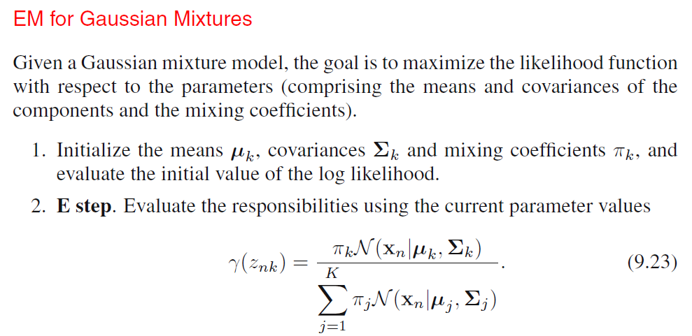
We can see that, \(\hat{\pi}_k, N_k, \boldsymbol{\hat{\mu}}_k, \boldsymbol{\hat{\Sigma}}_k\) all depends on the value of \(\gamma(Z_{nk})\) and \(\gamma(Z_{nk})\) depends on the values of all other variables. Thus, we can do a simple iterative scheme for finding a solution to the maximum likelihood problem, which turns out to be an instance of the EM algorithm for the particular case of Gaussian Mixture Model:

1. We first choose some initial values for the means, covariances and mixing coefficients.
2. We alternate between E step and M step:
   • Expectation Step: We use the current values for the parameters to evaluate the posterior probabilities (responsibilities).
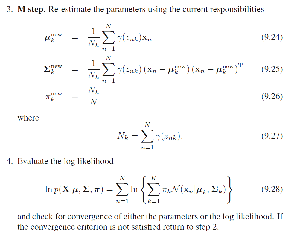
   • Maximization Step: We then use responsibilities to maximize the log likelihood function for parameters (Mean first, then covariance matrix).

In practice, the algorithm is deemed to have converged when the change in the log likelihood function or alternatively in the parameters falls below some threshold.

An Alternative View of EM

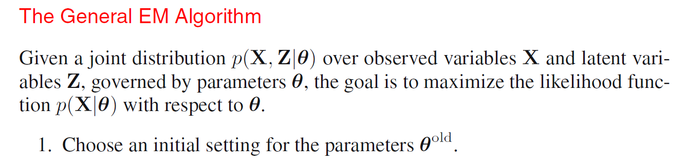
The goal of EM Algorithm is to find maximum likelihood solutions for models having latent variables. We denote sthe set of all observed data by \(\mathbf{D}\) in which the \(n\)th row represents \(\mathbf{x}^T_n\), and similarily we denote the set of all latent variables by \(\mathbf{H}\) with a corresponding row \(\mathbf{Z}^T_n\). The set of all parameters is denoted by \(\boldsymbol{\theta}\) and so the log likelihood function is given by:

\[\ln L(\boldsymbol{\theta}; \; \mathbf{D}) = \ln(\sum_{\mathbf{H}} P(\mathbf{D}, \mathbf{H} | \boldsymbol{\theta}))\]

If we have continuous latent variable, we can replace the summation by integral.

A key observation is that the summation over the latent variables appears inside the logarithm which provides much complicated expression of log likelihood. Suppose, for each observation in \(\mathbf{D}\), we have observed corresponding random variable \(\mathbf{Z}^T_n = \mathbf{z}^T_n\). We call \(\{\mathbf{D}, \mathbf{H}\}\) the complete dataset and if we only observed \(\mathbf{D}\) we have incomplete dataset, the maximization of this complete-data log likelihood function is straightforward and much simpler than incomplete likelihood.

In practice, we are not given the complete dataset but only the incomplete data. Our state of knowledge of the values of the latent variables in \(\mathbf{H}\) is given only by the posterior distribution:

\[P(\mathbf{H} | \mathbf{D}, \boldsymbol{\theta}) = \frac{P(\mathbf{H}, \mathbf{D} | \boldsymbol{\theta})}{P(\mathbf{D} | \boldsymbol{\theta})}\]

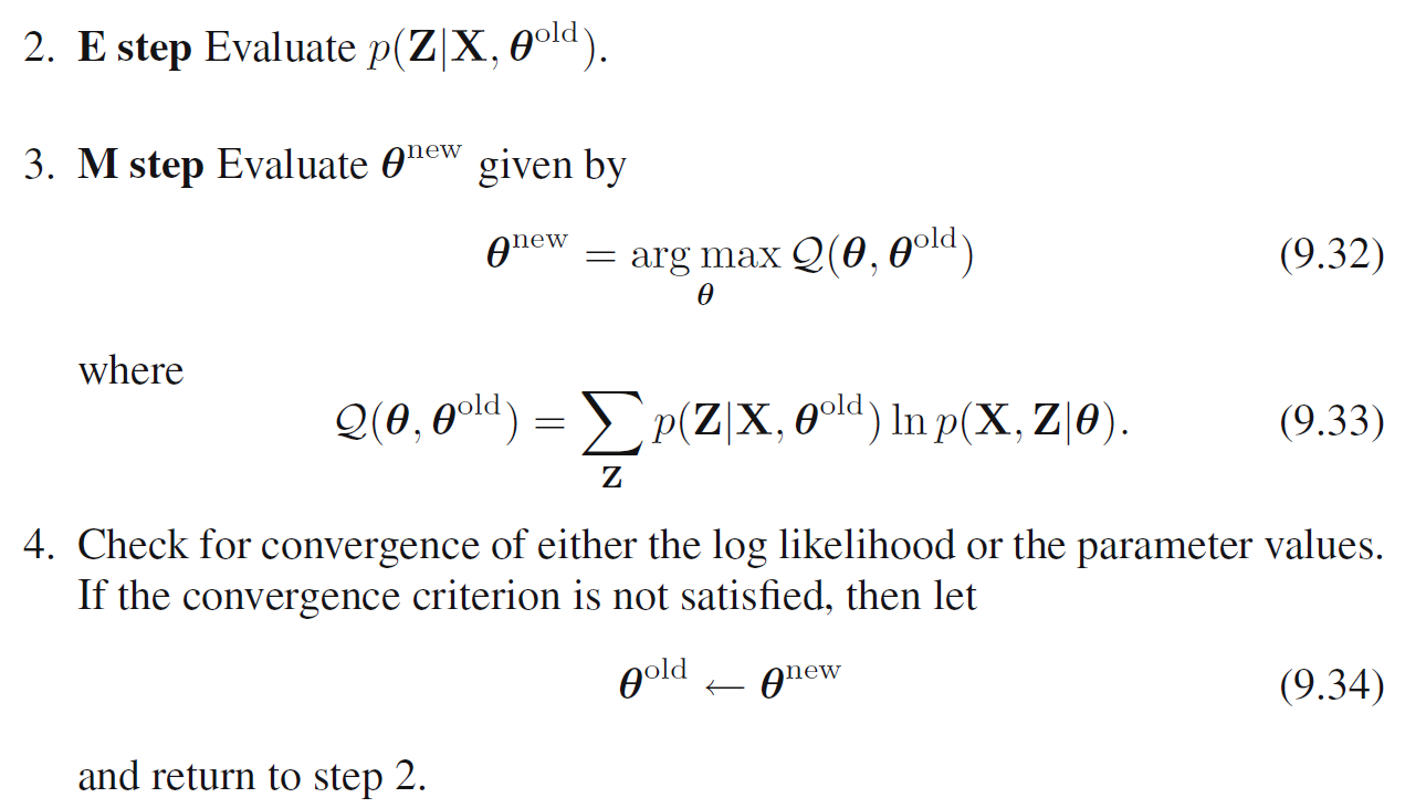
Since we cannot use the complete dataset log likelihood, we can consider using the expectation under the posterior distribution (E step). In E step, we use the current parameter values \(\boldsymbol{\theta}^{old}\) to find the posterior distribution of the latent variables given by \(P(\mathbf{H} | \mathbf{D}, \boldsymbol{\theta})\). We then use this posterior distribution to find the expectation of the complete-data log likelihood evaluated for some general parameter value \(\boldsymbol{\theta}\). This expectation, denoted as:

\[Q(\boldsymbol{\theta}, \boldsymbol{\theta}^{old}) = E_{\mathbf{H} | \mathbf{D}, \boldsymbol{\theta}^{old}} [\ln P(\mathbf{D}, \mathbf{H} | \boldsymbol{\theta})] = \sum_{\mathbf{H}} P(\mathbf{H} | \mathbf{D}, \boldsymbol{\theta}^{old}) \ln P(\mathbf{D}, \mathbf{H} | \boldsymbol{\theta})\]

In the subsequent M step, we find parameters that maximize this expectation. If the current estimate for the parameters is denoted \(\boldsymbol{\theta}^{old}\), then a pair of successive E and M steps gives rise to a revised estimate \(\boldsymbol{\theta}^{new}\). The algorithm is initialized by choosing some starting value for the parameters \(\boldsymbol{\theta}_0\).

\[\theta^{new} = \underset{\boldsymbol{\theta}}{\arg\max} \; Q(\boldsymbol{\theta}, \boldsymbol{\theta}^{old})\]

Notice here we have complete data log likelihood, compare it with incomplete data log likelihood, the log likelihood function is much easier to compute.

General EM algorithm

General EM Algorithm for Gaussian Mixture

Previously, we used incomplete data log likelihood for Gaussian Mixture together with the EM algorithm, we have summation over \(k\) over \(k\) that occurs inside the logarithm. Now, we try to use general approach of EM algorithm.

We have the complete data likelihood:

Where \(Z_{nk}\) is the \(k\) the component of \(\mathbf{Z}_n\). Taking the logarithm, we have the log likelihood:

\[\ln P(\mathbf{D}, \mathbf{H} | \boldsymbol{\mu}, \boldsymbol{\Sigma}, \boldsymbol{\pi}) = \sum^{N}_{n=1}\sum^{K}_{k=1} Z_{nk} (\ln \pi_k + \ln N(\mathbf{x}_n | \boldsymbol{\mu}_k, \boldsymbol{\Sigma}_k))\]

Compare with the incomplete data log likelihood, we can see that this form is much easier to solve. In practice, we do not obtain the values of \(\mathbf{H}\), thus, we use expectation instead:

We then proceed as follows:

1. First we start at some initial values for parameters.
2. We use these parameters to evaluate the responsibilities.
3. We then maximize the expected log likelihood function.

Which is the same as the incomplete data log likelihood EM previously, but we have a much easier log likelihood function to maximize over.

Ref

PRML Chapter 9

AdaBoost (Discrete)

Consider a two-class problem, with the output variable coded as \(Y \in \{-1, 1\}\). Given a vector of input variables \(\mathbf{X}\), a classifier \(G(\mathbf{X})\) produces a prediction taking one of the two values \(\{-1, 1\}\).

Suppose we have samples \(D = \{(\mathbf{x}_1, y_1), ...., (\mathbf{x}_N, y_N); \; \mathbf{x} \in \mathbb{R}^d\}\). The error rate (misclassification) on the training sample is defined as:

\[\bar{err} = \frac{1}{N} \sum^{N}_{i=1} I[y_i \neq G(\mathbf{x}_i)]\]

The expected error rate is defined as:

\[E_{X, Y} [I[Y \neq G(\mathbf{X})]]\]

A weak classifier is one whose error rate is only slightly better than random guessing. The purpose of boosting is to sequentially apply the weak classification algorithm to repeatedly modified versions of the data, thereby producing a sequence of weak classifiers \(G_{m} (\mathbf{x}), \; m = 1, ...., M\)

The predictions from all of them are then combined through a weighted majority vote to produce the final prediction:

\[G(x) = sign (\sum^{M}_{m=1} \alpha_m G_m (\mathbf{x}))\]

Here, \(\alpha_1, ...., \alpha_M\) are parameters that weight the contribution of each corresponding classifier \(G(\mathbf{x})\) and they are learned by the algorithm. They are here to give higher influence to the more accurate classifiers in the sequence.

The data modifications at each boosting step consist of applying weights \(w_1, ...., w_N\) to each of the training observations \((\mathbf{x}_i, y_i), \; i=1, ....., N\):

1. Initially all of the weights are set to \(w_i = \frac{1}{N}\), so the first step simply trains the classifier on the data in usual manner.
2. For each successive iteration \(m = 2, 3, .... , M\), the observation weights are individually modified:
   • Observations that were misclassified by the classifier \(G_{m-1} (\mathbf{x})\) induced at the previous step have their weights increased.
   • Observations that were classified correctly by the previous classifier have their weights decreased.
3. Then the classification algorithm is reapplied to the weighted observations

So misclassified samples have their weights increased so that each successive classifier is thereby forced to concentrate on those samples.

At each iteration \(m\):

1. A normalized weighted error rate (high penalty for misclassifying high weight samples)\(err_m\) is calculated.
2. The error rate is transformed by \(\log (\frac{1 - error_m}{error_m})\):
   • This function goes to positive infinity as \(error_m\) goes to 0
   • This function goes to negative infinity as \(error_m\) goes to 1 (we should just predict class inversely)
   • This function is 0 when error rate is 0.5
3. The new weight update:
   • If correctly classified, then we simply keep the original weight for the sample (It will be smaller because we are weighting it by sum of error rate in the next classifier).
   • If incorrectly classified:
     • If error rate is small, then \(\alpha\) is positively large so each misclassified sample's weight is increased
     • If error rate is high, then \(\alpha\) goes to negative infinity, so each misclassified sample's weight is decreased because this sample is correctly classified inversely so we decrease its weight.
     • If error rate is 0.5, then \(\alpha\) is 0, so each misclassified sample's weight is maintained

Boosting Fits an Additive Model

Boosting is a way of fitting an additive expansion in a set of elementary basis functions. Here the basis functions are the individual classifiers \(G_m(\mathbf{x}) \in \{-1, 1\}\). More generally, basis function expansions take the form:

\[f(\mathbf{x}) = \sum^{M}_{m=1} \beta_m b(\mathbf{x}; \boldsymbol{\gamma}_m)\]

Where \(\beta_m, \; m=1, 2, ...., M\) are the expansion coefficients, and \(b(\mathbf{x}; \gamma) \in \mathbb{R}\) are usually simple functions of multivariate argument \(\mathbf{x}\) characterized by a set of parameters \(\{\boldsymbol{\gamma}_1, ...., \boldsymbol{\gamma}_M\}\).

Typically these models are fit and the parameters are found by minimizing a loss function averaged over the training data:

\[\min_{ \{\beta_m, \boldsymbol{\gamma}_m\}^{M}_1 }\sum^{N}_{i=1} L(y_i, \sum^{M}_{m=1} \beta_m b(\mathbf{x}_i; \boldsymbol{\gamma}_m))\]

Forward Stagewise Additive Modeling

How to solve the above optimization problem? We can use forward stagewise modeling (greedy) to approximate the solution to above equation by sequentially adding new basis functions to the expansion without adjusting the parameters and coefficients of those that have already been added.

The loss function of optimization problem at each step \(m\) can be rewritten as:

\[L(y_i, f_m(\mathbf{x}_i)) = L(y_i, f_{m-1} (\mathbf{x}_i) + \beta b(\mathbf{x}_i; \boldsymbol{\gamma}))\]

Using the square loss, we have:

\[L(y_i, f_m(\mathbf{x}_i)) = (y_i - f_{m-1} (\mathbf{x}_i) - \beta b(\mathbf{x}_i; \boldsymbol{\gamma}))^2\]

\[\implies L(y_i, f_m(\mathbf{x}_i)) = (\epsilon_{im-1} - \beta b(\mathbf{x}_i; \boldsymbol{\gamma}))^2\]

This implies that we are fitting a basis function at each step to minimizing the residual from the current model \(f_{m-1} (\mathbf{x})\).

AdaBoost as Forward Stagewise Additive Modeling

Let the loss function be the exponential function:

\[L(y_i, f(\mathbf{x}_i)) = e^{-y_i f(\mathbf{x}_i)}\]

For adaboost, the basis functions are individual weak classifier \(G_m(x) \in \{-1, 1\}\). Using the exponential loss for additive stagewise modeling, we must minimize the objective:

\[(\beta_m, G_m) = \underset{\beta, G}{\arg\min} \sum^{N}_{i=1} e^{-y_i(f_{m-1} (\mathbf{x}_i) + \beta G(\mathbf{x}_i))}\]

Let \(w^{(m)}_i = e^{-y_i \mathbf{x}_i}\), then the above optimization can be expressed as:

\[(\beta_m, G_m) = \underset{\beta, G}{\arg\min} \sum^{N}_{i=1} w^{(m)}_i e^{-y_i\beta G(\mathbf{x}_i)}\]

Since, \(w^{(m)}_i\) does not depend on \(\beta, G(\mathbf{x})\), so it is just some constant and can be regard it as weight. Since this weight depends on previous prediction and current label, it is changing at each iteration \(m\).

Solve for \(\beta\)

In order to solve for \(\beta\), we can rewrite the objective as:

by taking the partial derivative w.r.t \(\beta\) and set it to 0:

\[\implies(e^\beta + e^{-\beta}) \sum_{i=1}^{N} w_i^{(m)}I(y_i \neq G(\mathbf{x}_i)) - e^{-\beta} \sum_{i=1}^{N} w_i^{(m)} = 0\]

\[\implies \frac{e^\beta + e^{-\beta}}{e^{-\beta}} = \frac{\sum_{i=1}^{N} w_i^{(m)}}{\sum_{i=1}^{N} w_i^{(m)}I(y_i \neq G(\mathbf{x}_i))}\]

\[\implies \frac{e^\beta}{e^{-\beta}} = \frac{\sum_{i=1}^{N} w_i^{(m)}}{\sum_{i=1}^{N} w_i^{(m)}I(y_i \neq G(\mathbf{x}_i))} - 1\]

\[\implies 2\beta = \log(\frac{1}{error_m} - 1)\]

\[\implies \beta_m = \frac{1}{2} \log (\frac{1 - error_m}{error_m})\]

Where \(error_m = \frac{\sum_{i=1}^{N} w_i^{(m)}I(y_i \neq G(\mathbf{x}_i))}{\sum_{i=1}^{N} w_i^{(m)}}\)

That is, for any classifier \(G\):

• \(\beta_m > 0\), if \(error_m < 0.5\)
• \(\beta_m < 0\), if \(error_m > 0.5\)

Solve for \(G\)

We want our basis function (weak classifier) to have better misclassification rate than random classifier, so we want \(error_m < 0.5\) which implies that we want \(\beta > 0\). Thus, for any value \(\beta > 0\), we can see that if we let \(G(\mathbf{x}_i) = y_i\) for all samples, we have minimum objective. Thus, we can transform the minimization problem to minimize the error rate:

By substitute \(G_m\) back to the solution of \(\beta\), we have:

\[\beta_m = \frac{1}{2} \log (\frac{1 - error_m}{error_m})\]

Where \(error_m = \frac{\sum_{i=1}^{N} w_i^{(m)}I(y_i \neq G_m(\mathbf{x}_i))}{\sum_{i=1}^{N} w_i^{(m)}}\)

The approximation is then updated:

\[f_m (\mathbf{x}_i) = f_{m-1} (\mathbf{x}_i) + \beta_m G_m (\mathbf{x}_i)\]

Which causes the weights for the next iteration to be:

Notice here, \(-y_i G_m (x_i) = 2 I[y_i \neq G_m (\mathbf{x}_i)] - 1\):

\[\implies w^{(m + 1)}_i = w^{(m)}_{i} e^{\alpha_m I[y_i \neq G_m(\mathbf{x}_i)]} e^{-\beta_m }\]

Where, \(\alpha_m = 2 \beta_m\) is the \(\alpha_m\) in Adaboost algorithm, and \(e^{-\beta_m}\) has no effect on weights because it is just a constant multiplying every sample.

Conclusion

Thus, we can think of Adaboost algorithm as stagewise additive modeling with basis function as a weak classifier (Minimizing the misclassification rate to have slightly better misclassification rate than random classifier) and exponential loss function.

Ref

ESLII Chapter 10

Random Forest

Bootstrap

Bagging

Earlier, we see that we can use bootstrap as a way of assessing the accuracy of a parameter estimate or a prediction. Here, we show how to use the bootstrap to improve the estimate or prediction itself.

Consider

Random Forest

Random Forests is a substantial modification of bagging that builds a large collection of de-correlated trees and then averages them. The essential idea in bagging is to average many noisy but approximately unbiased models and hence reduce the variance. Trees are ideal candidates for bagging, since they can capture complex interaction structures in the data, and if grown sufficiently deep, have relatively low bias. Since trees are notoriously noisy, they benefit greatly from the averaging (variance reduction).

Since each tree generated in bagging is identically distributed, the expectation of an average of \(B\) such tres is the same as the expectation of any one of them, this means the bias of bagged trees is the same as that of the individual trees and the only hope is the variance reduction. This is contrast to boosting, where the trees are grown in an adaptive way to remove bias, and hence are not identically distributed.

An average of \(B\) i.i.d random variables each with variance \(\sigma^2\), has variance \(\frac{1}{B} \sigma^2\). If the variables are simply i.d (not necessarily independent) with positive pairwise correlation \(\rho\), the variance of the average is:

\[\rho \sigma^2 + \frac{1 - \rho}{B} \sigma^2\]

As \(B\) increases, the second term disappears, but the first remains, and hence the size of the correlation of paris of bagged trees limits the benefits of averaging. The idea in random forest is to improve the variance reduction of bagging by reducing the correlation between the trees without increasing the variance too much. This is achieved in the tree-growing process through random selection of the input variables.

Specifically, when growing a tree on a bootstrapped dataset:

• Before each split, select \(m \leq p\) of the input variables at random as candidates for splitting (typically values for \(m\) are \(\sqrt{p}\) or even as low as 1)
• After \(B\) such trees \(\{T(\mathbf{x};\; \Theta_b)\}^{B}_{b=1}\) are grown, the random forest regression predictor is: \[\hat{f}^B_{rf} (\mathbf{x}) = \frac{1}{B}\sum^{B}_{b=1} T(\mathbf{x};\; \Theta_b)\]
• For classification, a random forest obtains a class vote from each tree, and then classifies using majority vote.

Out of Bag Samples

An importance feature of random forest is its use of out-of-bag samples:

• For each observation \(\mathbf{z}_i = (\mathbf{x}_i, y_i)\), construct its random forest predictor by averaging only those trees corresponding to bootstrap samples in which \(\mathbf{z}_i\) did not appear.

An out-of-bag error estimate (If short of data, it can be used as validation error) is almost identical to that obtained by \(N\)-fold cross validation, so unlike many other nonlinear estimators, random forest can be fit in one sequence, with cross-validation being performed along the way. Once the OOB error stabilizes, the training can be terminated.

Variable Importance

Random forests also use the OOB samples to construct a different variable-importance measure, apparently to measure the prediction strength of each variable. When the \(b\)th tree is grown, the OOB samples are passed down the tree, and the prediction accuracy is recorded. The values for the \(j\)th variable are randomly permuted in the OOB samples, and the accuracy is again computed. The decrease in accuracy as a result of this permuting is averaged over all trees, and is used as a measure of the importance of variable \(j\) in the random forest.

Overfitting

It is certainly true that increasing \(B\) does not cause the random forest sequence to overfit. like bagging, the random forest estimate approximates the expectation:

\[\hat{f}_{rf} (\mathbf{x}) = E[T(\mathbf{x}; \; \Theta)] = \lim_{B \rightarrow \infty} \hat{f}(\mathbf{x})^B_{rf}\]

with an average over \(B\) realizations of \(\Theta\). However, this limit can overfit the data, the average of fully grown trees can result in too rich a model and incur unnecessary variance. One possible solution is to reduce tree depth.

K-Means

Considering the problem of identifying groups, or clusters of data points in a multidimensional space.

Suppose we have a dataset \(\mathbf{x}_1, ....., \mathbf{x}_N\) consisting of \(N\) observations of a random \(D\) dimensional euclidean variable \(\mathbf{x}\). Our goal is to partition these points in to \(K\) clusters.

A cluster \(k\) contains:

1. Cluster center: \(\boldsymbol{\mu}_k \in \mathbb{R}^{D}\).
2. Assignment indicator variables: \(\mathbf{r}_{n} \in \mathbb{R}^{K}, \; r_{nk} \in \{0, 1\}\), one for each data point and each dimension \(k\) indicates whether the data point \(\mathbf{x}_n\) belongs to cluster \(k\)

So we can reformulate our goal to be: find an assignment of data points to clusters, as well as a set of cluster centers \(\{\boldsymbol{\mu}_k\}^{K}_{k=1}\), such that the sum of squares of the distances of each data point to its closest cluster center is a minimum. In equation, our objective is:

\[J(\mathbf{x}; \; \{\boldsymbol{\mu}_{k}, \mathbf{r}_{nk}\}) = \sum^{N}_{n=1}\sum^{K}_{k=1} r_{nk} \|\mathbf{x}_n - \boldsymbol{\mu}_k\|^2_2\]

Where the distance measure here is the L2 norm.

Thus, we want to find parameters \(\{\boldsymbol{\mu}_{k}, \mathbf{r}_{nk}\}\) such that the objective is minimized.

Algorithm

1. Initialize \(\boldsymbol{\mu}_k, \; \forall \; k=1, ...., K\)
2. Given \(\{\boldsymbol{\mu}_k\}\), minimize \(J\) w.r.t \(\{\mathbf{r}_{n}\}\)
3. Given \(\{\mathbf{r}_{n}\}\), minimize \(J\) w.r.t \(\{\boldsymbol{\mu}_k\}\)
4. Repeat 2, 3 until converges

For phase 2:

Given the cluster centers, it is obvious that if we assign each point to the closest cluster center, we have the minimum objective:

\[ r_{nk}= \begin{cases} 1, \quad \text{if }\; k = \underset{k}{\arg\min} \|\mathbf{x}_n - \boldsymbol{\mu}_k\|^2_2\\ 0, \quad o.w\\ \end{cases} \]

For phase 3:

Given the assignments, since the objective is convex, we can take gradient and solve for the optimal \(\boldsymbol{\mu}_k\):

\[\frac{\partial J}{\partial \boldsymbol{\mu}_k} = \sum^{N}_{n=1} -2 r_{nk} \mathbf{x}_n + 2\boldsymbol{\mu}_k \sum^{N}_{n=1} r_{nk} = 0\]

\[\implies \boldsymbol{\mu}_k \sum^{N}_{n=1} r_{nk} = \sum^{N}_{n=1} r_{nk} \mathbf{x}_n\]

\[\implies \boldsymbol{\mu}_k = \frac{\sum^{N}_{n=1} r_{nk} \mathbf{x}_n}{\sum^{N}_{n=1} r_{nk}}\]

\(\sum^{N}_{n=1} r_{nk} \mathbf{x}_n\) is the sum of all points that belongs to cluster \(k\) and \(\sum^{N}_{n=1} r_{nk}\) is the count of points in cluster \(k\), so the new \(\boldsymbol{\mu}_k\) is just the sample mean of the points in cluster \(k\).

Convergence

Since:

1. \(\{\boldsymbol{\mu}_{k}, \mathbf{r}_{nk}\}\) can only take finite values (i.e they are derived from finite subsets of data and uniquely defined for each subset).
2. At each step, we minimize the objective (i.e we either decrease or maintain the objective).
3. The cost function is bounded below zero.
4. Ties are broken consistently.

Thus, the algorithm can only take a finite number of non-decreasing steps before terminating at a local minimum.

Implementation

1
2
3
4
5
6
7
8
9
10
11
12
13
14
15
16
17
18
19
20
21
22
23
24
25
26
27
28
29
30
31
32
33
34
35
36
37
38
39
40
41
42
43
44
45
46
47
48

import numpy as np


class KMeans:
    def __init__(self, k=2, max_iteration=10, init_method='random'):
        self.k = k
        self.max_iteration = max_iteration
        self.init_method = init_method

    def fit_transform(self, x: np.array):
        n, d = x.shape
        curr_mu = self._init_mu(x)
        curr_iter = 0

        while curr_iter <= self.max_iteration:
            r_matrix = np.zeros((n, self.k))
            # step one, map each instance to cluster center muk
            for sample in range(n):
                distance = []
                for j in range(self.k):
                    distance.append(np.linalg.norm(x[sample] - curr_mu[j]))

                mu_assigned = np.argmin(distance)
                r_matrix[sample][mu_assigned] = 1
                
            # step two calculate new mu_k
            prev_mu = curr_mu.copy()
            for j in range(self.k):
                curr_mu[j] = np.mean(x[r_matrix[:, j] == 1], axis=0)
                
            # check stopping criteria
            if np.linalg.norm(prev_mu - curr_mu) == 0:
                break

            curr_iter += 1
            
        print(f'finished k-means algorithm, on iteration {curr_iter}')
        return r_matrix, curr_mu

    def _init_mu(self, x):
        if self.init_method == 'random':
            col_max = x.max(axis=0)
            col_min = x.min(axis=0)
            return (col_max - col_min) * np.random.random_sample((self.k, x.shape[1])) + col_min
        
        elif self.init_method == 'random_points':
            random_int = np.random.randint(0, x.shape[0], size=self.k)
            return x[random_int]

Principal Component Analysis

Let \([\mathbf{X}_1 ... \mathbf{X}_N]\) be a \(p \times N\) matrix of random sample where \(\mathbf{X}_i \in \mathbb{R}^p\). The sample mean \(\mathbf{M}\) of the random sample is defined as:

\[\mathbf{M} = \frac{1}{N} \sum^{N}_{i=1} \mathbf{X}_{i}\]

Let \(\hat{\mathbf{X}}_k\) be the centered random vector for \(k = 1, ...., N\):

\[\hat{\mathbf{X}}_k = \mathbf{X}_k - \mathbf{M}\]

Then we can defined the centered random sample matrix as:

\[B = [\hat{\mathbf{X}}_1 ... \hat{\mathbf{X}}_N]_{[p\times N]}\]

The sample covariance matrix \(S\) is then:

\[S = [\frac{1}{N} BB^T]_{[p\times p]}\]

We can easily show that \(S\) is positive semi-definite. Assume that \(\mathbf{x} > 0\):

Let \(\mathbf{A} = B^T\mathbf{x}\), then:

\[\frac{\mathbf{A}^T \mathbf{A}}{\mathbf{x}^T \mathbf{x}} = \lambda\]

Since, \(\mathbf{A}^T \mathbf{A} \geq 0\) for any vector \(A\), similar for \(\mathbf{x}^T \mathbf{x}\), then:

\[\lambda \geq 0\]

Since, \(S\) is symmetric and \(\lambda \geq 0\) for all eigenvalues of \(S\), we can conclude that \(S\) is positive semi-definite.

The total variance in the data is:

\[tr(S)\]

PCA

The goal of PCA is to find an orthogonal \(p \times p\) matrix \(P = [\mathbf{u}_1 .... \mathbf{u}_p]\) that determines a change of variable, \(\mathbf{X} = P\mathbf{Y}\) with the property that the features of \(\mathbf{Y}\) are uncorrelated and are arranged in order of decreasing variance.

Assume the \(\mathbf{X}\) is already being centered, that is \(B = [\mathbf{X}_1 .... \mathbf{X}_N]\), then \(\mathbf{Y}\) is also centered since \(P \neq 0\):

\[E[\mathbf{X}] = P\cdot E[\mathbf{Y}] = 0\]

Then the sample covariance matrix of \(\mathbf{Y}\) is:

\[S_Y = \frac{1}{N-1}[P^{-1}\mathbf{X}_1 .... P^{-1}\mathbf{X}_N] [P^{-1}\mathbf{X}_1 .... P^{-1}\mathbf{X}_N]^T\]

\[\implies S_{\mathbf{Y}} = \frac{1}{N-1} P^{T}BB^{T}P = P^{T} S_{\mathbf{X}} P\]

So the desired orthogonal matrix is the one that makes \(\hat{Cov}[Y_i, Y_j] = 0, \; \forall i \neq j\) (features are uncorrelated), which means that the we want the sample covariance matrix \(S_Y\) to be diagonal.

Let \(D\) be a diagonal matrix with eigenvalues of \(S_{\mathbf{X}}\), \(\lambda_1 ,...., \lambda_p\) on the diagonal s.t \(\lambda_1 \geq \lambda_2 \geq ..... \lambda_p \geq 0\), let \(P\) be an orthogonal matrix whose columns are the corresponding unit eigenvectors \(\mathbf{u}_1, ....., \mathbf{u}_p\) (Symmetric matrices have property that the eigenspaces are mutually orthogonal, in the sense that eigenvectors corresponding to different eigenvalues are orthogonal). Then, we can use \(P\) and \(\mathbf{X}\) to represent \(Y\), and the sample covariance matrix is:

\[S_{\mathbf{X}} = PDP^T \implies P^{-1} S_{\mathbf{X}} P = D\]

Thus, \(S_{\mathbf{Y}} = D\).

Then, the eigenvectors \(\mathbf{u}_1, ...., \mathbf{u}_p\) are called Principal Components of the data. The first PC is the eigenvector corresponding to the largest eigenvalue of \(S_{\mathbf{X}}\).

The result transformation is defiend as:

\[P^{T} \mathbf{X} = \mathbf{Y}\]

\[ \mathbf{Y} = \begin{bmatrix} \mathbf{u}^T_1 \mathbf{X} \\ .\\ .\\ .\\ \mathbf{u}^T_p \mathbf{X}\\ \end{bmatrix} \]

Total Variance

It can be shown that the PCA transformation does not change the total variance of the data, that is the total variance of the data is the sum of eigenvalues:

\[tr(S_{\mathbf{Y}}) = tr(D)\]

This is only true when we are dealing with sample covariance matrix,

Implementation

1
2
3
4
5
6
7
8
9
10
11
12
13
14
15

import numpy as np
def pca(X, k=2):
    u, s, vt = np.linalg.svd(X, full_matrices=False)
    xv = u * s

    return xv[:, :k]

def normalize(X):
    n, d = X.shape
    x_trans = X.copy()
    for j in range(d):
        # normalization
        x_trans[:, j] = (X[:, j] - X[:, j].mean()) / X[:, j].std()

    return x_trans

Ref

https://stats.stackexchange.com/questions/266864/why-is-the-sum-of-eigenvalues-of-a-pca-equal-to-the-original-variance-of-the-dat