Support Vector Machine

Given dataset $D=\{({\mathbf{x}}_1,y_1).....,({\mathbf{x}}_N,y_N);\mathbf{x}\in {\mathbb{R}}^m,y_i\in \{-1,1\}\}$. Let ${\mathbf{w}}^T\mathbf{x}+b=0$ be a hyperplane, we classify a new point ${\mathbf{x}}_i$ by

$${\hat{y}}_i({\mathbf{x}}_i)=\{\begin{array}{l}{\mathbf{w}}^T{\mathbf{x}}_i+b\ge 0,1\\ {\mathbf{w}}^T{\mathbf{x}}_i+b<0,-1\end{array}$$

Suppose that our data is linear separable. Then, $\mathrm{\exists }$ at least one possible combination of parameters $\{\mathbf{w},b\}$, such that:

$${\hat{\gamma }}_i=y_i{\hat{y}}_i({\mathbf{x}}_i)>0,\mathrm{\forall }i=1,....,N$$

When $y_i=1$, a confident classifier would have ${\hat{y}}_i({\mathbf{x}}_i)$ as large as possible. On the other hand, when $y_i=-1$, the confident classifier would have ${\hat{y}}_i({\mathbf{x}}_i)$ as negative as possible. Thus, we want ${\hat{\gamma }}_i$ as large as possible, this ${\hat{\gamma }}_i$ is called functional margin associated with training example for specific set of parameters $\{\mathbf{w},b\}$. And functional margin of $\{\mathbf{w},b\}$ is defined as minimum of these functions margins:

$$\hat{\gamma }=\underset{i=1,...,N}{min}{\hat{\gamma }}_i$$

In support vector machines the decision boundary is chosen to be the one for which the functional margin (confidence) is maximized.

Distance to Plane

Let ${\mathbf{x}}_i$ be a sample that has label $y_i=1$, thus, it is on the positive side of the hyperplane ${\mathbf{w}}^T\mathbf{x}+b=0$. Define $r$ to be the shortest distance between point ${\mathbf{x}}_i$ and the hyperplane. Then $r$ is the distance between ${\mathbf{x}}_i$ to its projection on the hyperplane ${\mathbf{x}}_i^{\prime }$.

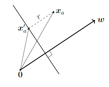
Since $\mathbf{w}$ is the normal vector that is orthogonal to the plane and $\frac{\mathbf{w}}{\Vert \mathbf{w}{\Vert }_2}$ is the unit vector that represents its direction. We can write the $r$ as:

$${\mathbf{x}}_i-{\mathbf{x}}_i^{\prime }=r\frac{\mathbf{w}}{\Vert \mathbf{w}{\Vert }_2}$$

$$⟹r=\frac{{\mathbf{x}}_i-{\mathbf{x}}_i^{\prime }}{\frac{\mathbf{w}}{\Vert \mathbf{w}{\Vert }_2}}$$

Goal

The concept of the margin is intuitively simple: it is the distance of the separating hyperplane to the closest examples in the dataset, assuming that our dataset is linearly separable. That is:

This optimization problem is unbounded, because one can make the functional margin large by simply scaling the parameters by a constant $c$, $\{c\mathbf{w},cb\}$:

$$y_i(c{\mathbf{w}}^T{\mathbf{x}}_i+cb)>y_i({\mathbf{w}}^T{\mathbf{x}}_i+b)=\hat{\gamma }$$

This has no effect on the decision plane because:

$${\mathbf{w}}^T{\mathbf{x}}_i+b=c{\mathbf{w}}^T{\mathbf{x}}_i+cb=0$$

Thus, we need to transform the optimization problem to maximize the distance between the samples and decision boundary instead of maximizing functional margin. Suppose we let all functional margins to be at least 1 (can easily achieve by multiplying parameters by a constant):

$$y_i({\mathbf{w}}^T{\mathbf{x}}_i+b)\ge 1$$

$$⟹{\mathbf{w}}^T{\mathbf{x}}_i+b\ge 1$$

$$⟹{\mathbf{w}}^T{\mathbf{x}}_i+b\le -1$$

Then, for point ${\mathbf{x}}_i$ on ${\mathbf{w}}^T{\mathbf{x}}_i+b=1$, we have its distance to the decision plane:

$${\mathbf{w}}^T{\mathbf{x}}_i+b-r\frac{\Vert \mathbf{w}{\Vert }_2^2}{\Vert \mathbf{w}{\Vert }_2}=0$$

$$⟹r=\frac{1}{\Vert \mathbf{w}\Vert }$$

Then, we can formulate our objective as:

Which is equivalent to:

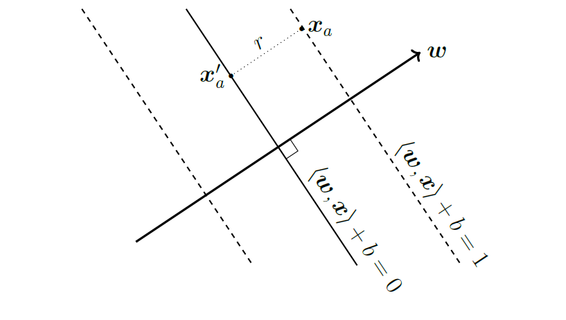
Soft Margin SVM

Slack Variables

Notice, in the above formulation, we have hard constraints on the margins which do not allow misclassification of points. However, in real world, data points are rarely linear separable and there will be outliers in the dataset, we may wish to allow some examples to be on the wrong side of the hyperplane or to have margin less than 1 .

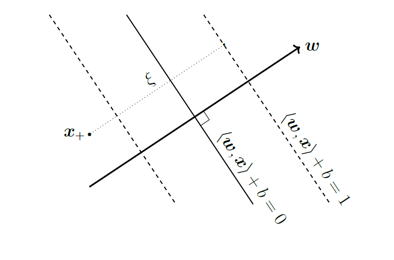
To resolve this problem, we can introduce slack variables one for each data point to relax the hard constraints:

$$y_i({\mathbf{w}}^T{\mathbf{x}}_i+b)\ge 1-{\xi }_i$$ $${\xi }_i\ge 0,\mathrm{\forall }i=1,....,N$$

To encourage correct classification of the samples, we add ${\xi }_i$ to the objective:

Thus, sample points are now permitted to have margin less than 1, and if an example ${\mathbf{x}}_i$ has slack variable greater than 0, we would have penalty in the objective function $C{\xi }_i$. The parameter $C$ controls the relative weighting between the twin goals of making the $\Vert \mathbf{w}\Vert$ small and of ensuring that most examples have functional margin at least 1.

Dual Problem

Using Lagrange Multiplier, we can transform the constrained problem into an unconstrained concave problem:

$$\underset{\mathit{\alpha },\mathit{\eta }}{max}\underset{\mathbf{w},b,\mathit{\xi }}{min}\frac{1}{2}\Vert \mathbf{w}{\Vert }_2^2+C\sum _{n=1}^N{\xi }_i-\sum _{i=1}^N{\alpha }_i[y_i({\mathbf{w}}^T{\mathbf{x}}_i+b)-1+{\xi }_i]-\sum _{i=1}^N{\eta }_i{\xi }_i$$

Where the inner minimization is the dual function and the maximization w.r.t $\alpha$ is called dual problem.

KKT

For an unconstrained convex optimization problem, we know we are at global minimum if the gradient is zero. The KKT conditions are the equivalent conditions for the global minimum of a constrained convex optimization problem. $\mathrm{\forall }i=1,....,N$:

1. Stationarity, If the strong duality holds, $({\mathbf{w}}^{\ast },{\mathit{\alpha }}^{\ast })$ is optimal, then ${\mathbf{w}}^{\ast }$ minimizes $L({\mathbf{w}}^{\ast },{\mathit{\alpha }}^{\ast })$ (same for $b^{\ast },{\xi }^{\ast }$ which are formulated as constraints in the dual problem):

   $${\mathrm{\nabla }}_{\mathbf{w}}L({\mathbf{w}}^{\ast },{\mathit{\alpha }}^{\ast })=0$$ $$⟹{\mathbf{w}}^{\ast }=\sum _{i=1}^n{\alpha }_i^{\ast }{y}_i{\mathbf{x}}_i$$

2. Complementary Slackness: $${\alpha }_i[y_i({\mathbf{w}}^T{\mathbf{x}}_i+b)-1+{\xi }_i]=0$$

3. Primal Feasibility: $$y_i({\mathbf{w}}^T{\mathbf{x}}_i+b)-1+{\xi }_i\ge 0$$ $${\eta }_i{\xi }_i=0$$

4. Dual Feasibility: $${\alpha }_i,{\eta }_i,{\xi }_i\ge 0$$

Solving Dual Problem

We now solve for the dual function by fixing $\{{\alpha }_i{\eta }_i\}$ (satisfying Stationarity condition):

$$\underset{\mathbf{w},b,\mathit{\xi }}{min}\frac{1}{2}\Vert \mathbf{w}{\Vert }_2^2+C\sum _{n=1}^N{\xi }_i-\sum _{i=1}^N{\alpha }_i[y_i({\mathbf{w}}^T{\mathbf{x}}_i+b)-1+{\xi }_i]-\sum _{i=1}^N{\eta }_i{\xi }_i$$

Substitute back to the original equation, we obtain the dual function:

$$g(\mathit{\alpha })=-\frac{1}{2}\sum _{i=1}^N\sum _{k=1}^N{\alpha }_i{\alpha }_k{{\mathbf{x}}_i}^T{\mathbf{x}}_k{y}_i{y}_k+\sum _{i=1}^N{\alpha }_i$$

Then, we have the dual problem:

This is a quadratic programming problem that we can solve using quadratic programming.

Interpretation

We could conclude:

1. if $0<{\alpha }_i<C⟹y_i(w^T{x}_i+b)=1-{\xi }_i$ Since ${\alpha }_i=C-{\mu }_i,{\mu }_i\ge 0$, we have ${\xi }_i=0⟹$ the points are with $0<{\alpha }_i<C$ are on the margin

2. if ${\alpha }_i=C$

   • $0<{\xi }_i<1$: the points are inside the margin on the correct side
   • ${\xi }_i=1$: the points are on the decision boundary
   • ${\xi }_i>1$: the points are inside the wrong side of the margin and misclassified

3. if ${\alpha }_i=0$, the points are not support vectors, have no affect on the weight.

After finding the optimal values for $\mathit{\alpha }$, we obtain optimal ${\mathbf{w}}^{\ast }$ by solving:

$${\mathbf{w}}^{\ast }=\sum _{i=1}^n{\alpha }_i^{\ast }{y}_i{\mathbf{x}}_i$$

We obtain optimal $b^{\ast }$ by realizing that the points on the margins have $0<{\alpha }_i<C$. Let ${\mathbf{x}}_i$ be one of those points, then:

$${{\mathbf{w}}^{\mathbf{\ast }}}^T{\mathbf{x}}_i+b=y_i$$

Let $M$ be the set of all points that lies exactly on the margin, a more stable solution is obtained by averaging over all points:

$$b^{\ast }=\frac{1}{N_m}\sum _{i=1}^{N_m}(y_i-{{\mathbf{w}}^{\mathbf{\ast }}}^T{\mathbf{x}}_i)$$

Kernel Tricks

Implementation

1
2
3
4
5
6
7
8
9
10
11
12
13
14
15
16
17
18
19
20
21
22
23
24
25
26
27
28
29
30
31
32
33
34
35
36
37
38
39
40
41
42
43
44
45
46
47
48
49
50
51
52
53
54
55
56
57
58
59
60
61
62
63
64
65
66
67
68
69

from cvxopt import matrix, solvers
import numpy as np
from qpsolvers import solve_qp
from sklearn.svm import SVC

class SVM:

    def __init__(self, c=1, kernel='linear'):
        self.c = c
        self.kernel = kernel
        self.b = None
        self.dual_coef_ = None
        self.decision_matrix = None

    def fit(self, X, y):
        n, d = X.shape
        y = y.reshape(-1, 1)
        yyt = np.matmul(y, y.T)
        P = np.zeros((n, n))
        q = matrix(-np.ones((n, 1)))
        a = matrix(y.T, tc='d')
        b = matrix([0.0])
        G = matrix(np.row_stack([np.diag([-1] * n), np.diag([1] * n)]), tc='d')
        h = matrix(np.row_stack([np.array([0] * n).reshape(n, 1),
                                 np.array([self.c] * n).reshape(n, 1)]), tc='d')
        for i in range(n):
            for j in range(n):
                P[i][j] = self.apply_kernel(X[i], X[j])

        P = matrix(P * yyt)
        alpha = np.array(solvers.qp(P, q, G, h , a, b)['x'])
        alpha[alpha < np.mean(alpha) * 0.1] = 0
        temp_x = np.column_stack([X, alpha, y])
        m = temp_x[(temp_x[:, -2] > 0) & (temp_x[:, -2] < self.c)]
        N_m = len(m)
        self.decision_matrix = m[:, :-2]
        self.b = 0
        self.dual_coef_ = m[:, -1] * m[:, -2]

        ## get b
        for i in range(N_m):
            self.b += m[i, -1]
            for j in range(N_m):
                self.b -= m[j, -2] * m[j, -1] * self.apply_kernel(m[i, :-2], m[j, :-2])

        self.b = self.b / N_m

        return self

    def apply_kernel(self, x_1, x_2):
        if self.kernel == 'linear':
            return np.dot(x_1, x_2)

    def decision_function(self, X):
        pred_results = np.array([])
        for i in range(len(X)):
            pred = self.b
            for j in range(len(self.decision_matrix)):
                pred += self.dual_coef_[j] * self.apply_kernel(X[i], self.decision_matrix[j])

            pred_results = np.append(pred_results, pred)

        return pred_results

    def predict(self, X):
        pred_results = self.decision_function(X)
        
        return np.where(pred_results >= 0, 1, -1)

Ref

https://www.ccs.neu.edu/home/vip/teach/MLcourse/6_SVM_kernels/lecture_notes/svm/svm.pdf

http://www.cs.cmu.edu/~guestrin/Class/10701-S06/Slides/svms-s06.pdf

MML book

Lagrangian Duality for Dummies, David Knowles

PRML Chapter 7

Naive Bayes

Suppose our training set consists of data samples $D=\{({\mathbf{x}}_1,y_1),....,({\mathbf{x}}_N,y_N)\},{\mathbf{x}}_{\mathbf{i}}\in {\mathbb{R}}^d$, where $D=\{({\mathbf{x}}_i,y_i)\}$ are realizations of a random sample that follows unknown joint distribution $P(\mathbf{X},Y)$.

Assumptions:

1. Features are conditionally independent (Naive bayes assumption): $$P(\mathbf{X}|Y)=\prod _{j=1}^{d}P(X_j|Y)$$

2. MLE assumption: Random sample is identically distributed.

3. Positional independence: The position of features does not matter (used in Multinomial case).

By applying bayes rule (applying on distribution $P(\cdot )$ to make things general), we have:

$$P(Y|\mathbf{X})=\frac{P(\mathbf{X},Y)}{P(\mathbf{X})}=\frac{P(\mathbf{X}|Y)P(Y)}{P(\mathbf{X})}$$

By substituting the assumption:

$$P(Y|\mathbf{X})=\frac{\prod _{j=1}^{d}P(X_j|Y)P(Y)}{P(\mathbf{X})}$$

Since the probability distribution $P(\mathbf{X})$ characterised by $F_{\mathbf{X}}(\mathbf{x})$ is constant for any given $\mathbf{x}$, we can drop it from the equation because it only changes $P(Y|\mathbf{X})$ by a proportion:

$$P(Y|\mathbf{X})\propto P(Y)\prod _{j=1}^{d}P(X_j|Y)$$

Our goal is to find a class $\hat{y}$ that maximize the probability given input $\mathbf{X}=\mathbf{x}$:

Logistic Regression

Suppose we have training examples $D=\{({\mathbf{x}}_1,y_1),....,({\mathbf{x}}_N,y_N);{\mathbf{x}}_i\in {\mathbb{R}}^d\}$, our goal is to make decision about the class of new input $\mathbf{x}$. The logistic regression does this by learning from a training set, a vector of bias and a matrix of weights.

Binary-Class

In binary class problem, our target $Y$ takes values $\{0,1\}$. To model the distribution $P(Y|\mathbf{X};\mathbf{w},b)$, we apply sigmoid function on the dot product of weights and inputs which transform the output to a value between $[0,1]$ (one criteria for probability):

$$z={\mathbf{x}}^T\mathbf{w}+b$$

$$y=\sigma (z)$$

To make sure that class random variable $Y$'s conditional pmf sums to 1:

$$P(Y=1|X=\mathbf{x};\mathbf{w},b)=\frac{1}{1+e^{-z}}=p$$

$$P(Y=0|X=\mathbf{x};\mathbf{w},b)=1-\frac{1}{1+e^{-z}}=\frac{e^{-z}}{1+e^{-z}}=1-p$$

Then, it is equivalently to express this conditional pmf as Bernoulli pmf:

$$p_{Y|\mathbf{X}}(y|\mathbf{x};\mathbf{w},b)=p^y+(1-p{)}^{1-y}$$

If we have the conditional pmf of $Y$ given $X=\mathbf{x}$, then we can use simple decision rule to make decisions:

$$\hat{y}=\{\begin{array}{l}P(Y=1|X=\mathbf{x})>0.5,1\\ P(Y=1|X=\mathbf{x})\le 0.5,0\end{array}$$

Gradient Boosting Decision Trees

Boosting Trees

Regression and classification trees partition the space of all joint predictor variable values into disjoint regions $R_j,j=1,2,....,J$ as represented by the terminal nodes of the tree. A constant $c_j$ is assigned to each such region and the prediction rule is:

$$\mathbf{x}\in R_j⟹f(\mathbf{x})=c_j$$

Thus, a tree can be formally expressed as:

$$T(\mathbf{x};\mathit{\theta })=\sum _{j=1}^J{c}_{j}I[\mathbf{x}\in R_j]$$

with parameters $\theta =\{R_j,c_j{\}}_1^J$. The parameters are found by iteratively solving minimizing problem:

1. Given $R_j$, we solve ${\hat{c}}_j$ by simply taking the average or majority class.
2. $R_j$ is found by iterating over all possible pairs of feature and splitting point.

The boosted tree model is a sum of such trees induced in a forward stagewise manner:

$$f_M(\mathbf{x})=\sum _{m=1}^{M}T(\mathbf{x};{\mathit{\theta }}_m)$$

At each step, one must solve:

$${\hat{\mathit{\theta }}}_m=\underset{{\mathit{\theta }}_m}{\arg min}\sum _{i=1}^{N}L(y_i,f_{m-1}({\mathbf{x}}_i)+T({\mathbf{x}}_i;{\mathit{\theta }}_m))$$

Gradient Boosting

In general, it is hard to directly take partial derivatives w.r.t the tree's parameters, thus, we take partial derivatives of tree predictions $f({\mathbf{x}}_i)$.

Fast approximate algorithms for solving the above problem with any differentiable loss criterion can be derived by analogy to numerical optimization. We first start with general case. The loss in using $\mathbf{f}$ to predict $y$ on the training data is:

$$L(\mathbf{f})=\sum _{i=1}^{N}L(y_i,f({\mathbf{x}}_i))$$

The goal is to minimize $L({\mathbf{x}}_i)$ w.r.t $f$, where here $f(\mathbf{x})$ is constrained to be a sum of trees $f_M(\mathbf{x})$.

We first start with general case where $f$ can be any parameters or numbers. In this case, we have $N$ samples, thus, $\mathbf{f}=\{f({\mathbf{x}}_1),....,f({\mathbf{x}}_N)\}\in {\mathbb{R}}^N$.

Then, the gradient of objective w.r.t $\mathbf{f}={\mathbf{f}}_{m-1}$ which is the current model is:

$${\mathbf{g}}_m={\mathrm{\nabla }}_{\mathbf{f}}L(\mathbf{f})=<\frac{\partial L(\mathbf{f})}{\partial f({\mathbf{x}}_1)},....,\frac{\partial L(\mathbf{f})}{\partial f({\mathbf{x}}_N)}>$$

Then this gradient points at the direction of steepest increase, it tells us how we can change our current predictions to increase our loss. Since we want to minimize the objective, we would like to adjust our current predictions to the direction of steepest decrease:

$${\mathbf{h}}_m=-{\rho }_m{\mathbf{g}}_m$$

Where ${\rho }_m$ is the step size for current model and it is minimizer of:

$${\rho }_m=\underset{\rho }{\arg min}L({\mathbf{f}}_{m-1}-\rho {\mathbf{g}}_m)$$

The current solution is then updated as

$${\mathbf{f}}_m=f_{m-1}-{\rho }_m{\mathbf{g}}_m$$

If fitting the training data (minimizing the loss) is our ultimate goal, then the above update rule can solve our problem by adding the negative gradient at each iteration. However, our ultimate goal is to generalize to new data, copying and pasting training data exactly is not what we want. One possible solution is to learn the update $-{\rho }_m{\mathbf{g}}_m$ by fitting a simple decision tree:

$${\hat{\mathit{\theta }}}_m=\underset{\mathit{\theta }}{\arg min}\sum _{i=1}^N(-g_{im}-T(x_i;\mathit{\theta }){)}^2$$

That is, we fit a regression tree $T$ to the negative gradient values.

Algorithm

1. We first start by a constant model (model that predict constants) which is a single terminal node tree.
2. For all samples new targets are generated to be the negative gradient of the loss function w.r.t the current model prediction ${\mathbf{f}}_{m-1}$.
3. Fit a regression tree to minimize the MSE between new target (negative gradient) and current prediction.

Discussions

Regularization

For numbers of gradient boosting rounds $M$, the loss can be made arbitrarily small. However, fitting the data too well can lead to overfitting which degrades the risk on future predictions.

Shrinkage

Controlling the value of $M$ is not the only possible regularization strategy, we can add penalty terms to the loss function that penalize large $M$ or we can weight subsequent trees. The simplest implementation of shrinkage in the context of boosting is to scale the contribution of each tree by a factor of $0<v<1$, when it is added to the current approximation:

$$f_m(\mathbf{x})=f_{m-1}(\mathbf{x})+v\sum _{j=1}^J{c}_{jm}I[\mathbf{x}\in R_{jm}]$$

The parameter $v$ can be regarded as controlling the learning rate of the boosting procedure. Smaller values of $v$ result in larger training error for the same number of iterations $M$ but might have better generalization. Thus, both $v$ and $M$ control prediction risk on the training data. $v$ and $M$ tradeoff each other, therefore in practice, it is best to set $v$ small and control $M$ by early stopping.

Subsampling

We know that bootstrap averaging (bagging) improves the performance of a noisy classifier through averaging (reduce variance). We can exploit the same idea in gradient boosting.

At each iteration, we sample a fraction $\eta$ of the training observations without replacement, and grow the next tree using that subsample. A typical value of $\eta$ is 0.5, although for large sample size $N$, we can have smaller $\eta$.

Ref

https://www.ccs.neu.edu/home/vip/teach/MLcourse/4_boosting/slides/gradient_boosting.pdf

Decision Trees (CART)

Tree based methods partition the feature space into a set of rectangles, and then fit a simple model (i.e constant) in each one. We focus on CART in this post.

Suppose we have dataset $D=\{({\mathbf{x}}_1,y_1),....,({\mathbf{x}}_N,y_N);{\mathbf{x}}_i\in {\mathbb{R}}^d\}$. The algorithm needs to automatically decide on the splitting variables and splitting points and also what shape the tree should have.

Regression Trees

In this scenario, our response variable $Y$ is continuous. Suppose first that we have a partition into $M$ regions $R_1,....,R_M$ and we define the model prediction as:

$$\hat{y}=\sum _{m=1}^M{c}_{m}I[{\mathbf{x}}_i\in R_m]$$

By minimizing the mean square loss $\frac{1}{2}\frac{1}{N}\sum _{i=1}^N(y_i-{\hat{y}}_i{)}^2$, we have:

Thus, the best estimate ${\hat{c}}_m$ in each region is the average training responses in that region w.r.t mean square error:

$${\hat{c}}_m=\frac{1}{N_m}\sum _{i=1}^N{y}_{i}I[{\mathbf{x}}_i\in R_m]$$

Where $N_m=\sum _{i=1}^{N}I[{\mathbf{x}}_i\in R_m]$, is total training examples in region $R_m$.

Heaps

The binary heap data structure is an array object that we can view as a nearly complete binary tree. Each node of the tree corresponds to an element of the array. The tree is completely filled on all levels except possibly the lowes, which is filled from the left up to a point that is the elements in the subarray $A[\lfloor \frac{n}{2}\rfloor +1...n]$ are all leaves.

An array $A$ that represents a heap is an object with two attributes:

1. $A.length$: gives the number of elements in the array. $A[1:A.length]$.
2. $A.heap\mathrm{\_}size$: gives how many elements in the heap are stored within array $A$. $A[1:A.heap\mathrm{\_}size:A.length]$

Given the index $i$ of a node, we can easily compute the indices of its parent, left child and right child by:

1. parent: $\lfloor \frac{i}{2}\rfloor$ (by shifting right 1 bit i >> 1)
2. left child: $2i$ (by shifting left 1 bit i << 1)
3. right child: $2i+1$ (by shifting left 1 bit and add 1 i << 1 + 1)

There are two types of binary heap:

1. Max heap: satisfies the max heap property that for every node $i$ other than the root $A[parent(i)]\ge A[i]$, that is the maximum value in the array is stored in the root and the subtree rooted at a node contains values no larger than that contained at the node itself (heap sorts).
2. Min heap: satisfies the min heap property that is organized in the opposite way, for every node $i$ other than the root $A[parent(i)\le A[i]]$ (priority queues)

1
2
3
4
5
6
7
8
9
10
11
12
13
14
15
16
17
18
19
20
21
22
23

class Heap:
    def __init__(self, A, heap_size):
        # A may not be a heap, call build_min_heap or build_max_heap to convert this instance to heap
        assert isinstance(A, list)
        self.heap_size = heap_size
        self.length = len(A)
        self._A = A
    
    def left(self, i):
        return i << 1
        
    def right(self, i):
        return i << 1 + 1

    def parent(self, i):
        return i >> 1
    
    def __getitem__(self, index):
        return self._A[index]
    
    def append(self, val):
        self._A.append(val)
        

Backpropagation In Convolutional Neural Networks

Cross Correlation

Given an input image $I$ and a filter $K$ of dimensions $k_1\times k_2$, then the cross correlation operation is defined as:

$$(I\otimes K{)}_{ij}=\sum _{m=0}^{k_2-1}\sum _{n=0}^{k_1-1}I(i+m,j+n)K(m,n)$$

Convolution

$$(I\ast K{)}_{ij}^d=\sum _{m=0}^{k_2-1}\sum _{n=0}^{k_1-1}I(i-m,j-n)K(m,n)$$

which is equivalent to cross correlation with flipped kernel (i.e flipped 180 degree)

$$(I\ast K{)}_{ij}=\sum _{m=0}^{k_2-1}\sum _{n=0}^{k_1-1}I(i+m,j+n){\text{ rot}}_{180}(K(m,n))$$

Statistics Inference

Sampling and Statistics

In a typical statistical problem, we have $p_X(x),f_X(x)$ unknown. Our ignorance about the $p_X(x),f_X(x)$ can roughly be classified in one of two ways:

1. $f(x)$ or $p_X(x)$ is completely unknown.
2. The form of $f_X(x)$ or $p_X(x)$ is known down to an unknown parameter vector $\theta$.

We will focus on the second case. We often denote this problem by saying that the random variable $X$ has density or mass function of the form $f_X(x;\theta )$ or $p_X(x;\theta )$, where $\theta \in \mathrm{\Omega }$ for a special parameter space $\mathrm{\Omega }$. Since $\theta$ is unknown, we want to estimate it.

In the process, our information about case 1 or 2 comes from a sample on $X$. The sample observations have the same distribution as $X$, and we denote them as $X_1,....,X_n$ where $n$ is the sample size. When the sample is actually drawn, we use lower case letters to represent the realization $x_1,...,x_n$ of random samples.

Once the sample is drawn, then $t$ is called the realization of $T$, where $t=T(x_1,....,x_n)$.

Value Function Approximation (Algorithms)

Approximate Value Iteration

Population Version

Recall that the procedure for VI is:

$$V_{k+1}\leftarrow T^{\pi }{V}_k$$ $$V_{k+1}\leftarrow T^{\ast }{V}_k$$

One way to develop its approximation version is to perform each step only approximately (i.e find $V_{k+1}\in \mathbf{F}$) such that:

$$V_{k+1}\approx T{V}_k$$

Where $T$ can be $T^{\ast }$ or $T^{\pi }$.

We start from a $V_0\in \mathbf{F}$, and then at each iteration $k$ of AVI, we solve (i.e $p$ is often 2):

$$V_{k+1}\leftarrow \underset{V\in \mathbf{F}}{\arg min}\Vert V-T{V}_k{\Vert }_{p,\mu }^p$$

At each iteration, $T{V}_k$ (our target) may not be within $\mathbf{F}$ anymore even though $V_k\in \mathbf{F}$, we may have some approximation error at each iteration of AVI. The amount of error depends on how expressive $\mathbf{F}$ is and how much $T$ can push a function within $\mathbf{F}$ outside that space.

Batch Version

The objective of AVI cannot be computed because:

• $\mu$ is unknown
• Environment $R,P$ is often not available, thus $T{Q}_k$ cannot be computed.

If we have samples in the form of $(X,A,R,X^{\prime })$, we can compute the unbiased sample of $T{Q}_k$:

$${\hat{T}}^{\pi }{Q}_k=R+\gamma Q(X^{\prime },A^{\prime })$$ $${\hat{T}}^{\ast }{Q}_k=R+\gamma \underset{a^{\prime }\in A}{max}Q(X^{\prime },a^{\prime })$$

Where $A^{\prime }\sim \pi (\cdot |X^{\prime })$

The question is: can we replace $T{Q}_k$ with $\hat{T}{Q}_k$?

Since $Z\sim \mu$:

Since the expectation of variance term does not depend on $Q$, the solution to the surrogate objective is the same as the original objective:

$$\underset{Q\in \mathbf{F}}{\arg min}{E}_{\mu ,\hat{T}{Q}_k}[|Q(Z)-\hat{T}{Q}_k(Z){|}^2]=\underset{Q\in \mathbf{F}}{\arg min}\Vert Q(Z)-T{Q}_k(Z){\Vert }_{2,\mu }^2$$

Similar to ERM, we do not know the environment dynamics $R,P$ and distribution $\mu$. We can use samples and estimate the expectation:

$$\frac{1}{N}\sum _{i=1}^N|Q(X_i,A_i)-\hat{T}{Q}_k(X_i,A_i){|}^2=\Vert Q-\hat{T}{Q}_k{\Vert }_{2,D_n}^2$$

This is the basis of DQN.

Bellman Residual Minimization

Population Version

Recall that:

$$V=T^{\pi }V⟹V=V^{\pi }$$

Under FA, we may not achieve this exact equality, instead:

$$V\approx V^{\pi }$$

Thus, we can formulate our objective:

$$V=\underset{V\in \mathbf{F}}{\arg min}\Vert V-T^{\pi }V{\Vert }_{p,\mu }^p=\Vert BR(V){\Vert }_{p,\mu }^p$$

By minimizing this objective ($p$ is usually 2), we have Bellman Residual Minimization.

This procedure is different from AVI in that we do not mimic the iterative process of VI (which is convergent in the exact case without any FA), but instead directly go for the solution of fixed-point equation ($V-T^{\pi }V$ instead of $V-T^{\pi }{V}_k$).

If there exists a $V\in \mathbf{F}$ that makes $\Vert V-T^{\pi }V{\Vert }_{2,\mu }^2=0$ and if we assume $\mu (x)>0,\mathrm{\forall }x\in \chi$, we can conclude that $V(x)=V^{\pi }(x),\mathrm{\forall }x\in \chi$ so $V=V^{\pi }$.

Batch Version

Similar to AVI, we may want to replace $TV$ or $TQ$ by $\hat{T}Q$. Thus, our empirical objective is:

$$Q=\underset{Q\in \mathbf{F}}{\arg min}\frac{1}{N}\sum _{i=1}^N|Q(X_i,A_i)-{\hat{T}}^{\pi }Q(X_i,A_i){|}^2=\Vert Q-{\hat{T}}^{\pi }Q{\Vert }_{2,D_n}^2$$

Using $D_n=\{(X_i,A_i,R_i,X_i^{\prime }){\}}_{i=1}^N$

We can see that $Q$ appears in both ${\hat{T}}^{\pi }Q$ and $Q$, which is different from AVI and ERM. This causes an issue: the minimizer of $\Vert Q-T^{\pi }Q{\Vert }_{2,\mu }^2$ and $\Vert Q-{\hat{T}}^{\pi }Q{\Vert }_{2,\mu }^2$ are not necessarily the same for stochastic dynamics.

To see this, for any $Q$ and $Z=(X,A)$ we compute:

$$E_{{\hat{T}}^{\pi }Q}[|Q(Z)-\hat{T}Q(Z){|}^2|Z]$$

Then:

Since $Z\sim \mu$, the first term is:

$$E_{{\hat{T}}^{\pi }Q,\mu }[|Q(Z)-T^{\pi }Q(Z){|}^2]=\Vert Q-T^{\pi }Q{\Vert }_{2,\mu }^2$$

The second term is:

$$E_{\mu }[E_{{\hat{T}}^{\pi }Q}[|T^{\pi }Q(Z)-{\hat{T}}^{\pi }Q(Z){|}^2|Z]]=E_{\mu }[Var[{\hat{T}}^{\pi }Q(Z)|Z]]$$

We can see that the variance term $Var[{\hat{T}}^{\pi }Q(Z)$ depends on $Q$, as we minimize the objective w.r.t $Q$ in stochastic dynamical systems (for deterministic ones, it is zero), we have $E_{}[Var{[}^{}Q(Z)|Z]]$, so the minimizer of the batch version objective is not the same as population version for BRM in stochastic dynamics.

Projected Bellman Error

From BRM, we know that even though $V\in \mathbf{F}$, $T^{\pi }V$ may not be in $\mathbf{F}$. Thus, a good approximator $V\in \mathbf{F}$ should have distance to $T^{\pi }V$ small. Thus, we want to find $V\in \mathbf{F}$ such that $V$ is the projection of $T^{\pi }V$ onto the space $\mathbf{F}$.

We want to find a $V\in \mathbf{F}$ such that:

$$V=\prod _{\mathbf{F},\mu }{T}^{\pi }V$$

Where $\prod _{\mathbf{F},\mu }$ is the projection operator.

TRhe projectio operator $\prod _{\mathbf{F},\mu }$ is a linear operator that takes $V\in B(\chi )$ and maps it to closest point on $F$ measured according to its $L_2(\mu )$ norm:

$$\prod _{\mathbf{F},\mu }V\triangleq \underset{V^{\prime }\in \mathbf{F}}{\arg min}\Vert V^{\prime }-V{\Vert }_{2,\mu }^2$$

It has some properties:

1. The projection belongs to function space $\mathbf{F}$: $$\prod _{\mathbf{F},\mu }V\in \mathbf{F}$$
2. If $V\in \mathbf{F}$, the projection is itself: $$V\in \mathbf{F}⟹\prod _{\mathbf{F},\mu }V=V$$
3. The projection operator onto a subspace is a non-expansion: $$\Vert \prod _{\mathbf{F},\mu }{V}_1-\prod _{\mathbf{F},\mu }{V}_2{\Vert }_{2,\mu }^2\le \Vert V_1-V_2{\Vert }_{2,\mu }^2$$

Population Version

We can define a loss function based on $V=\prod _{\mathbf{F},\mu }{T}^{\pi }V$:

$$\Vert V-\prod _{\mathbf{F},\mu }{T}^{\pi }V{\Vert }_{2,\mu }^2$$

This is called Projected Bellman Error or Mean Square Projected Bellman Error.

We find the value function by solving the following optimization problem:

$$V=\underset{V\in \mathbf{F}}{\arg min}\Vert V-\prod _{\mathbf{F},\mu }{T}^{\pi }V{\Vert }_{2,\mu }^2$$

Since $V\in \mathbf{F}$, the projection operator is linear: