Addressing Function Approximation Error in Actor-Critic Methods
As in function approximation with discrete action space, overestimation property also exists in continuous control setting.
Background
The return is defined as the discounted sum of rewards:
\[R_t = \sum^{T}_{i=t} \gamma^{i - t} r(s_i, a_i)\]
The objective of RL is to find the optimal policy \(\pi_{\phi}\) with parameters \(\phi\) which is defined as:
\[J(\phi) = E_{s_i \sim P_{\pi_\phi}, a_i \sim \pi_{\phi}} [R_0]\]
In DPG, the policy's (actor) parameter can be updated:
\[\nabla_{\phi} J(\phi) = E_{s_i \sim \rho_{\pi_\phi}} [\nabla_{\phi} \pi_{\phi} \nabla_{a} Q^{\pi_{\phi}} (s, a) |_{a = \pi_{\phi}(s)}]\]
Where the critic is the action value function:
\[Q^{\pi_{\phi}} (s, a) = E_{s_i \sim P_{\pi_{\phi}}, a_i \sim \pi_{\phi}}[R_t | s, a] = \underbrace{r}_{\text{ reward is deterministic so the expectation is itself }} + \gamma E_{s^{\prime}, a^{\prime}} [Q^{\pi} (s^{\prime}, a^{\prime}) | s, a]\]
In large state space, the critic can be approached using FA methods for example DQN (Approximate value iteration) in an off policy fashion (replay buffer):
\[Q_{k + 1} = {\arg\min}_{Q} \|Q - \hat{T}^{\pi_{\phi}} Q_{k}\|^2_{\rho_{\pi_{\phi}}}\]
with \(Q_{k}\) parameterized by a target network \(Q_{\theta^{\prime}}\), so the target \(\hat{T}^{\pi_{\phi}} Q_{\theta^{\prime}}\) can be write as:
\[\hat{T}^{\pi_{\phi}} Q_{\theta^{\prime}} = r + \gamma Q_{\theta^{\prime}} (s^{\prime}, a^{\prime}), \quad \quad a^{\prime} \sim \pi_{\phi} (\cdot | s^{\prime})\]
In terms of DDPG with delayed parameters to provide stability, the delayed target \(\hat{T}^{\pi_{\phi^{\prime}}} Q_{\theta^{\prime}}\) is used instead:
\[\hat{T}^{\pi_{\phi^{\prime}}} Q_{\theta^{\prime}} = r + \gamma Q_{\theta^{\prime}} (s^{\prime}, a^{\prime}), \quad \quad a^{\prime} \sim \pi_{\phi^{\prime}} (\cdot | s^{\prime})\]
The weights of a target network are either updated periodically to exactly match the weights of the current network or by some portion as in DDPG.
Overestimation Bias
In Q-learning with discrete actions, if the target is susceptible to error \(\epsilon\), then the maximum over the value alonge with its error will generally be greater than the true maximum even the error \(\epsilon\) has zero mean:
\[E_{\epsilon} [\max_{a^{\prime}} (Q(s^{\prime}, a^{\prime}) + \epsilon)] \geq \max_{a^{\prime}} Q(s^{\prime}, a^{\prime})\]
This issue extends to actor critic setting where policy is updated via gradient descent.
Overestimation Bias in Actor-Critic
Assumptions:
- Policy is updated using DPG.
- \(Z_1, Z_2\) are chosen to normalize the gradient (i.e \(Z^{-1} \|E[\cdot]\| = 1\), only provides direction)
Given current policy parameters \(\phi\), let:
\(\phi_{approx}\) be the parameters from the actor update induced by the maximization of the approximate critic \(Q_{\theta} (s, a)\). The resulting policy is \(\pi_{approx}\). \[\phi_{approx} = \phi + \frac{\alpha}{Z_1} E_{s \sim \rho_{\pi_{\phi}}} [\nabla_{\phi} \pi_{\phi} \nabla_{a} Q_{\theta} (s, a) |_{a = \pi_{\phi}(s)}]\]
\(\phi_{true}\) be the parameters from the hypothetical actor update with respect to the true underlying value function \(Q^{\pi_{\phi}} (s, a)\) (which is unknown during training). The resulting policy is \(\pi_{true}\). \[\phi_{true} = \phi + \frac{\alpha}{Z_2} E_{s \sim \rho_{\pi_{\phi}}} [\nabla_{\phi} \pi_{\phi} \nabla_{a} Q^{\pi_{\phi}} (s, a) |_{a = \pi_{\phi}(s)}]\]
Since gradient always point at the direction of maximum increase locally, so:
\(\exists \epsilon_1\), such that if \(\alpha \leq \epsilon_1\), then the approximate value of \(\pi_{approx}\) will be bounded by the approximate value of \(\pi_{true}\): \[E[Q_{\theta} (s, \pi_{approx} (s))] \geq E[Q_{\theta} (s, \pi_{true} (s))]\]
\(\exists \epsilon_2\), such that if \(\alpha \leq \epsilon_2\), then the true value of \(\pi_{approx}\) will be bounded by the true value of \(\pi_{true}\): \[E[Q^{\pi_{\phi}} (s, \pi_{true} (s))] \geq E[Q^{\pi_{\phi}} (s, \pi_{approx} (s))]\]
If: \[E[Q_{\theta} (s, \pi_{true} (s))] \geq E[Q^{\pi_{\phi}} (s, \pi_{true} (s))]\]
which means in expectation the approximated value function is greater than the true value function w.r.t policy \(\pi_{true}\) (e.g for some state action pair (\(s, \pi_{true} (s)\))), the approximate value is much larger than the true value). At the same time, if \(\alpha < \min(\epsilon_1, \epsilon_2)\), then: \[E[Q_{\theta} (s, \pi_{approx} (s))] \geq E[Q^{\pi_{\phi}} (s, \pi_{approx} (s))]\]
This implies that our policy improvement based on approximate value function would over-estimate certain actions and lead to sub-optimal policies.
Consequences of overestimation:
- Overestimation may develop into a more significant bias over many updates if left unchecked.
- Inaccurate value estimate may lead to poor policy updates.
Feedback loops of actor and critic is prone to overestimation because suboptimal actions may highly rated by suboptimal critic and reinforcing the suboptimal action in the next policy update.
Clipped Double Q-learning for Actor-Critic (Solution)
In DDQN, the target is estimated using the greedy action from current value network rather than current target network. In an actor-critic setting (DPG), the update is:
\[y = r + Q_{\theta^{\prime}} (s^{\prime}, \pi_{\phi} (s^{\prime}))\]
However, slow-changing policy in actor-critic, the current and target networks were too similar to make an independent estimation and offered little improvement.
Instead, we can go back and use similar formulation as Double Q-learning with a pair of actors \((\pi_{\phi_1}, \pi_{\phi_2})\) and critics \((Q_{\theta_1}, Q_{\theta_2})\) where \(\pi_{\phi_1}\) is optimized w.r.t \(Q_{\phi_1}\) and \(\pi_{\phi_2}\) is optimized w.r.t \(Q_{\phi_2}\):
\[y_1 = r + \gamma Q_{\theta^{\prime}_2} (s^{\prime}, \pi_{\phi_1} (s^{\prime}))\] \[y_2 = r + \gamma Q_{\theta^{\prime}_1} (s^{\prime}, \pi_{\phi_2} (s^{\prime}))\]
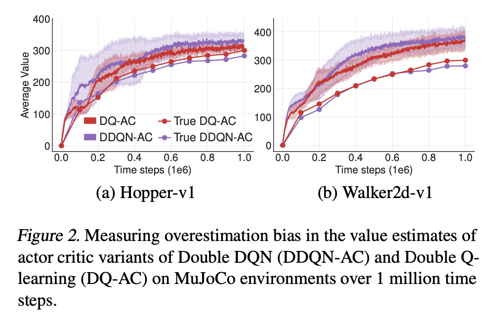
From above plot we can see that Double Q-learning AC is more effective, but it does not entirely eliminate the over-estimation. One cause can be the shared replay buffer, as a result, for some state \(s\), we would have \(Q_{\theta_2} (s, \pi_{\phi_1} (s)) > Q_{\theta_1} (s, \pi_{\phi_1} (s))\). This is problematic because we know that \(Q_{\theta_1} (s, \pi_{\phi_1} (s))\) will generally overestimate the true value, the overestimation is exaggerated.
One solution is to simply upper-bound the less biased value estimate \(Q_{\theta_2}\) by the biased estimate \(Q_{\theta_1}\):
\[y_1 = r + \gamma \min_{i=1, 2} Q_{\theta^{\prime}_{i}} (s^{\prime}, \pi_{\phi_1} (s^{\prime}))\]
This algorithm is called Clipped Double Q-learning algorithm. With Clipped Double Q-learning, exaggeration of overestimation is eliminated. However, underestimation bias could occur.
In implementation, computational costs can be reduced by using a single actor optimized w.r.t \(Q_{\theta_1}\). We then use the same target \(y_2=y_1\) for \(Q_{\theta_2}\). If \(Q_{\theta_2} > Q_{\theta_1}\) then the update is identical to the standard update and induces no additional bias. If \(Q_{\theta_2} < Q_{\theta_1}\), this suggests overestimation has occurred.
Addressing Variance
Besides impact on overestimation bias, high variance estimates provide a noisy gradient for the policy update which reduces learning speed and hurt performance in practice.
Since we never really learn \(Q^{\pi}\) exactly (we learn \(Q_{\theta}\) instead), there will always be some TD error in each update :
\[\begin{aligned}
r + \gamma E[Q_{\theta} (s^{\prime}, a^{\prime}) | s, a] - E[\delta(s, a) | s, a] &= \gamma E[Q_{\theta} (s^{\prime}, a^{\prime}) | s, a] - \gamma E[Q_{\theta} (s^{\prime}, a^{\prime}) | s, a] + Q_{\theta} (s, a)\\
&= Q_{\theta} (s, a)
\end{aligned}\]
Then:
\[\begin{aligned}
Q_{\theta} (s_t, a_t) &= r_t + \gamma E[Q_{\theta} (s_{t+1}, a_{t+1}) | s_t, a_t] - E[\delta_{t} | s_t, a_t]\\
&= r_t + \gamma E[r_{t+1} + \gamma E[Q_{\theta} (s_{t+2}, a_{t+2}) | s_{t+1}, a_{t+1}] - E[\delta_{t+1} | s_{t+1}, a_{t+1}] | s_t, a_t] - E[\delta_{t} | s_t, a_t]\\
& = E_{s_i \sim P_{\pi}, a_i \sim \pi} [\sum^{T}_{i=t} \gamma^{i - t} (r_i - \delta_i)]
\end{aligned}\]
Thus, the value function we estimate \(Q_{\theta} (s_t, a_t)\), approximates the expected return minus the expected discounted sume of future TD-errors instead of the expected return \(Q^{\pi}\).
If the value estimate (sample of \(Q_{\theta}\)) is a function of future reward and estimation error, it follows that the variance of the estimate will be proportional to the variance of future reward and estimation error. If the variance for \(\gamma^{i} (r_i - \delta_i)\) is large, then the accumulative variance will be large especially when gamma is large.
Target Networks and Delayed Policy Updates
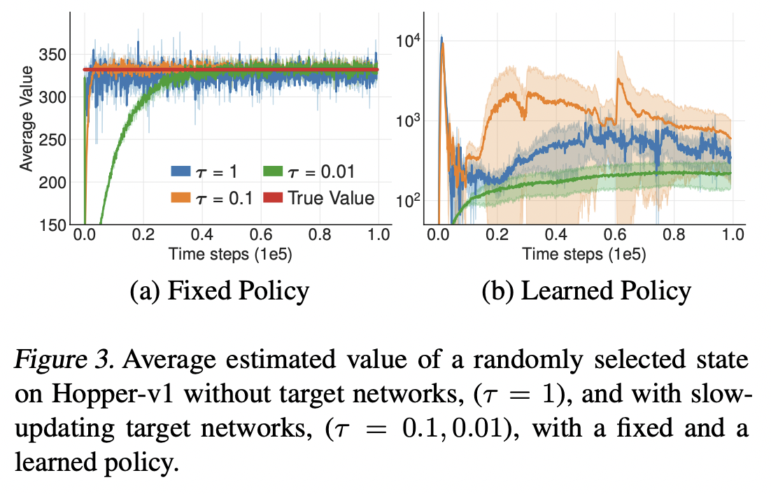
One way to reduce the estimation error is to delay each update to the target network. Consider the graph above:
- If \(\tau = 1\), we obtain batch semi-gradient TD algorithm for updating the critic, which may have high variance.
- If \(\tau < 1\), we obtain approximate value iteration.
If target networks can be used to reduce the error over multiple updates, and policy updates on high-error states cause divergent behavior, then the policy network should be updated at a lower frequency than the value network, to first minimize error before introducing a policy update.
Thus, delaying policy updates can be helpful in minimizing the estimation error by updating the policy and target networks after a fixed number of updates \(d\) to the critic. To ensure the TD-error remains small, target network is also slowly updated by \(\theta^{\prime} \leftarrow \tau \theta + (1 - \tau) \theta^{\prime}\).
Target Policy Smoothing Regularization
Since deterministic policies can overfit to narrow peaks in the value estimate, a regularization strategy is used for deep value learning, target policy smoothing which mimics the learning update from SARSA. The idea is that similar actions should have similar value (reduce the variance of target):
\[y = r + E_{\epsilon} [Q_{\theta^{\prime}} (s^{\prime}, \pi_{\phi^{\prime}} (s^{\prime}) + \epsilon)]\]
In practice, we can approximate this expectation over actions (\(\pi_{\phi^{\prime}} (s^{\prime}) + \epsilon\)) by adding a small amount of random noise to the target policy and averaging over mini-batches:
\[y = r + \gamma Q_{\theta^{\prime}} (s^{\prime}, \pi_{\phi^{\prime}} (s^{\prime}) + \epsilon)\]
\[\epsilon \sim clip(N(0, \sigma), -c, c)\]
Where noise is clipped to have it close to the original action (make sure it is a small area around original action).
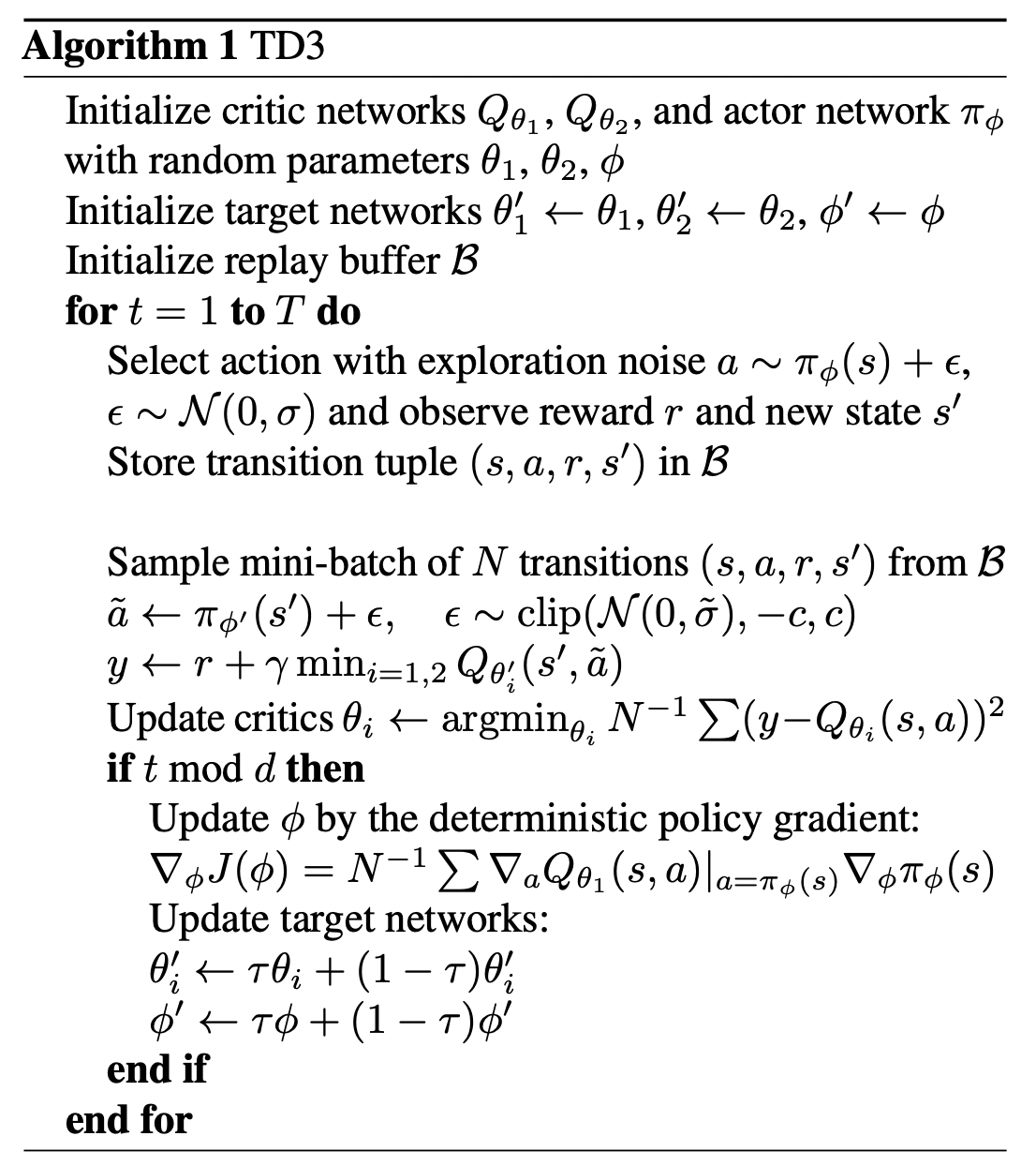
Algorithm
Conclusion
The paper focus on resolve overestimation error in actor critic setting (DPG) and discusses that failure can occur due to the interplay between the actor and critic updates. Value estimates diverge through overestimation when the policy is poor, and the policy will become poor if the value estimate itself is inaccurate (high variance).
Solutions:
Overestimation Error in value estimation: using clipped double Q-learning to estimate the target value \(y_1, y_2\) \[y_1 = r + \gamma \min_{i=1, 2} Q_{\theta^{\prime}_{i}} (s^{\prime}, \pi_{\phi^{\prime}} (s^{\prime}))\] \[y_2 = y_1\]
Estimation Error (TD error) and High Variance in value estimation: By using delayed policy and value updates with target networks, we have more stable and more accurate estimate of the value function by updating the value function several times.
Overfitting in Value estimation: by forcing the value estimate to be similar for similar actions, we smooth out the value estimation. \[y = r + \gamma Q_{\theta^{\prime}} (s^{\prime}, \pi_{\phi^{\prime}} (s^{\prime}) + \epsilon)\] \[\epsilon \sim clip(N(0, \sigma), -c, c)\]
The general structure of the algorithm follows DDPG.