Delving Deep into Rectifiers: Surpassing Human-Level Performance on ImageNet Classification

PReLU

Parametric Rectifiers

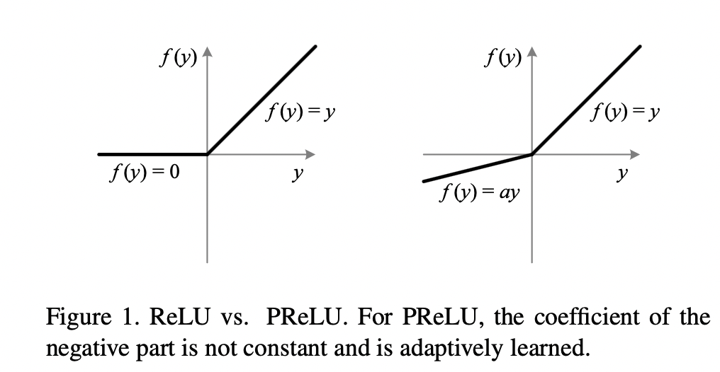
Formally, we consider an activation function defined as: \[ f(y_i)= \begin{cases} y_i, \quad & y_i > 0\\ a_i y_i, \quad & y_i \leq 0\\ \end{cases} \]

Here \(y_i\) is the input of the nonlinear activation \(f\) on the \(i\)th channel, and \(a_i\) is a coefficient controlling the slop of the negative part of the function. The subscript \(i\) in \(a_i\) indicates that we allow the nonlinear activation to vary on different channels. When \(a_i = 0\), it becomes ReLU. When \(a_i\) is small and fixed value, we have LReLU. When \(a_i\) is a learnable parameter, we call this Parametric ReLU (PReLU).

ImageNet Classification with Deep Convolutional Neural Networks

The dataset, Image preprocessing

ImageNet is a dataset of over 15 million labeled high-resolutoin images. It consists of variable-resolution images, while the network requires a constant input dimensionality. Therefore, we down-sampled the images to a fixed resolution of \(256 \times 256\). Given a rectangular image, we first rescaled the image such that the shorter side was of length 256, and then cropped out the central \(256 \times 256\) patch from the resulting image. We did not pre-process the images in any other way, except for subtracting the mean activity over the training set for each pixel (normalize each input pixel). So we trained our network on the centered raw RGB values of the pixels.

题目库: [1688， 79, 78, 46, 22, 90, 47, 39, 40, 93, 53, 70, 121, 122, 118, 392, 62, 198, 5, 55, 64, 322, 63, 120, 93, 45 213, 343, 300, 279, 1143, 494, 152, 518, 377, 416, 309, 337, 221, 139, 119, '面试题17.16', 746, 376]

Backtracking

1688 Easy

1
2
3
4
5
6
7
8
9
10
11
12
13
14

class Solution:
    def numberOfMatches(self, n: int) -> int:
        def find_matches(n):
            if n == 1:
                return 0
            else:
                if n % 2 == 0:
                    counts = find_matches(n // 2)
                else:
                    counts = find_matches(n // 2 + 1) 
                
                return counts + n // 2
            
        return find_matches(n)

Actor-Critic Algorithms

Original Paper

Trees

1
2
3
4
5
6
7
8
9
10

class BinaryTreeNode:
    def __init__(self, key=None, left=None, right=None, p=None):
        self.key = key
        self.left = left
        self.right = right
        self.p = p

class BinarySearchTree:
    def __init__(self, root=None):
        self.root = root

Binary Search Tree

A binary search tree node consists of:

1. \(key: \;\) value of the node
2. \(left: \;\) left children
3. \(right: \;\) right children
4. \(p: \;\) parent

If a child or the parent is missing, the appropriate attribute contains the value None. The root node is the only node in the tree whose parent is None.

The keys in a binary search tree are always stored in such a way as to satisfy the binary search tree property:

For any node \(x\), the keys in the left subtree of \(x\) are at most \(x.key\), and the keys in the right subtree of \(x\) are at least \(x.key\).

The binary search tree property allows us to print out all the keys in a binary search tree in sorted order by inorder tree walk (Inorder traversal). This algorithm prints the key of the root of a subtree betweeen printing the values in its left subtree and printing those in its right subtree. Similarly, a preorder tree walk prints the root before the values in either subtree and a postorder tree walk prints the root after the values in its subtrees.

Inorder Traversal

1
2
3
4
5
6
7
8
9
10
11

def inorder_tree_walk(tree):

    def inorder(root):
        if not root:
            return
        
        inorder(root.left)
        print(root.val)
        inorder(root.right)
        
    inorder(tree)

Preorder Traversal

1
2
3
4
5
6
7
8
9
10
11

def preorder_tree_walk(tree):

    def preorder(root):
        if not root:
            return
        
        print(root.val)
        preorder(root.left)
        preorder(root.right)
        
    preorder(tree)

Postorder Traversal

1
2
3
4
5
6
7
8
9
10
11

def postorder_tree_walk(tree):

    def postorder(root):
        if not root:
            return
        
        postorder(root.left)
        postorder(root.right)
        print(root.val)
        
    postorder(tree)

Search

We use the following procedure to search for a node with a given key in a binary search tree. Given a pointer to the root of the tree and a key \(k\), it returns a pointer to a node with key \(k\) if one exists, otherwise it returns None.

1
2
3
4
5
6
7
8
9
10
11
12
13
14
15

def tree_search(tree, k):
    
    def search(root, val):
        # base case
        if not root or root.key == val:
            return root
        
        if root.key < val:
            target = search(root.right, val)
        else:
            target = search(root.left, val)
        
        return target
    
    return search(tree, k)

Minimum

We can always find an element in a binary search tree whose key is a minimum by following \(left\) child pointers from the root until we encounter a None. The following procedure returns a pointer to the minimum element in the subtree rooted at a given node \(x\):

1
2
3
4
5
6
7
8
9
10

def tree_minimum(tree):
    
    def minimum(root):
        # base case
        if not root.left:
            return root
        
        return minimum(root.left)
    
    return minimum(tree)

Maximum

The maximum is symmetric as minimum:

1
2
3
4
5
6
7
8
9
10

def tree_maximum(tree):
    
    def maximum(root):
        # base case
        if not root.right:
            return root
        
        return maximum(root.right)
    
    return maximum(tree)

Successor and Predecessor

Given a node in a binary search tree, sometimes we need to find its successor in the sorted order determined by an inorder tree walk. If all keys are distinct, the successor of a node \(x\) is the node with the smallest key greater than \(x.key\). The procedure breaks into several cases:

1. If node \(x\) has right subtree, then the successor must be the smallest element in the right subtree.
2. If node \(x\) does not have right subtree and itself is a leftsubtree of its parent, then the successor must be its parent.
3. If node \(x\) does not have right subtree and itself is a rightsubtree of its parent, then the successor must be the lowest ancestor of \(x\) whose left child is also an ancestor of \(x\).

1
2
3
4
5
6
7
8
9
10
11
12
13
14
15

def tree_successor(node):
    # case 1
    if node.right:
        return tree_minimum(node)
    
    # case 2, 3
    curr_p = node.p
    while curr_p:
        if curr_p.left == node:
            return curr_p
        
        node = curr_p
        curr_p = node.p
        
    return None

Predecessor is symmetric

Insertion

To insert a new node \(z\) into a binary search tree \(T\) we use the following procedure:

1. Begin at root of the tree, we maintain two pointers \(y, x\) representing parent and current node respectively.
2. Go down the tree and compare every node encounter with \(z\), if it is greater than \(z\) we go to the left, if smaller we go to the right, until we reach None.
3. We replace \(y.left\) or \(y.right\) with \(x\) and fill \(z.p = y\).

1
2
3
4
5
6
7
8
9
10
11
12
13
14
15
16
17
18
19
20

def tree_insert(T, z):
    # initialize y, x representing parent and current node
    y, x = None, T
    # step 2
    while x:
        y = x
        if z.key < x.key:
            x = x.left
        else:
            x = x.right
    
    # step 3
    z.p = y
    # if tree is empty
    if not y:
        T.root = z
    elif z.key < y.key:
        y.left = z
    else:
        y.right = z

Deletion

The overall strategy for deleting a node \(z\) from a binary search tree \(T\) has three basic cases:

1. If \(z\) has no children, then we can simply remove it by modifying its parent to replace \(z\) with None as its child.
2. If \(z\) has just on child, then we elevate that child to take \(z\)'s position in the tree by modifying \(z\)'s parent to replace \(z\) by \(z\)'s child.
3. If \(z\) has two children, then we find \(z\)'s successor \(y\) which must be the minimum item in \(z\)'s right subtree (with no left child). Now have two cases:
   1. If \(y\) is \(z\)'s right child: We replace \(z\) by \(y\) and \(z\)'s left child becomes \(y\)'s left child.
   2. If \(y\) is not \(z\)'s right child: We first replace \(y\) by its right child, then we replace \(z\) by \(y\)

In order to move subtrees around, we define a helper function transplant that replaces the subtree rooted at node \(u\) with the subtree rooted at node \(v\).

1
2
3
4
5
6
7
8
9
10
11
12
13
14
15
16
17
18
19
20
21
22
23
24
25
26
27
28
29
30
31
32
33
34

def transplant(T, u, v):
    # if u is the root
    if not u.p:
        T.root = v
    elif u.p.left == u:
        u.p.left = v
    else:
        u.p.right = v

    # replace v with u
    if v:
        v.p = u.p

def tree_delete(T, z):
    # case 1
    if not z.left and not z.right:
        transplant(T, z, None)
    # case 2
    elif not z.left and z.right:
        transplant(T, z, z.right)
    elif not z.right and z.left:
        transplant(T, z, z.left)
    else:
        y = tree_successor(z)
        # case 3.2
        if z.right != y:
            transplant(T, y, y.right)
            y.right = z.right
            y.right.p = y
            
        transplant(T, z, y)
        y.left = z.left
        y.left.p = y
    

Complexcity

• Tree walks: \(\; \Theta(n)\)
• Search, Minimum, Maximum, Successor, Predecessor, Insert, Delete: \(\; O(h)\)

Search

Breath First Search

Breadth First Search (BFS) algorithm traverses a graph in a breadthward motion and uses a queue to remember to get the next vertex to start a search, when a dead end occurs in any iteration.

As in the example given above, BFS algorithm traverses from A to B to E to F first then to C and G lastly to D. It employs the following rules:

• Visit the adjacent unvisited vertex. Mark it as visited. Display it. Insert it in a queue.
• If no adjacent vertex is found, remove the first vertex from the queue, and set this vertex as the head.
• Repeat Rule 1 and Rule 2 until the queue is empty.

1
2
3
4
5
6
7
8
9
10
11
12
13
14
15
16
17
18
19
20
21
22
23
24

class BinaryTreeNode:
    def __init__(self, key=None, parent=None, left_child=None, right_child=None):
        self.key = key
        self.parent = parent
        self.left_child = left_child
        self.right_child = right_child

class Tree:
    def __init__(self, tree=None):
        self.root = tree

def bfs(tree):
    from collections import deque
    q = deque()
    q.append(tree)
    while q:
        head = q.popleft()
        print(head.key)
        if head.left_child:
            q.append(head.left_child)
            
        if head.right_child:
            q.append(head.right_child)

Depth First Search

Depth First Search (DFS) algorithm traverses a graph in a depthward motion and uses a stack to remember to get the next vertex to start a search, when a dead end occurs in any iteration.

As in the example given above, DFS algorithm traverses from S to A to D to G to E to B first, then to F and lastly to C. It employs the following rules:

• Visit the adjacent unvisited vertex. Mark it as visited. Display it. Push it in a stack.
• If no adjacent vertex is found, pop up a vertex from the stack. (It will pop up all the vertices from the stack, which do not have adjacent vertices.)
• Repeat Rule 1 and Rule 2 until the stack is empty.

1
2
3
4
5
6
7
8
9
10
11
12
13
14
15
16
17
18
19
20
21

def dfs(tree):
    if not tree.left_child and not tree.right_child:
        print(tree.key)
    else:
        print(tree.key)
        if tree.left_child:
            dfs(tree.left_child)
        
        if tree.right_child:
            dfs(tree.right_child)

def dfs_stack(tree):
    stack = [tree]
    while stack:
        head = stack.pop()
        print(head.key)
        if head.right_child:
            stack.append(head.right_child)
        
        if head.left_child:
            stack.append(head.left_child)

Reference

https://www.tutorialspoint.com/data_structures_algorithms/depth_first_traversal.htm

Value Function Approximation (Introduction)

In real-world problem, the state space \(\chi\) or the state-action space \(\chi \times A\) is large that we cannot represent quantities such as the value function or policy exactly.

• \(\chi \subseteq \mathbb{R}^d\) with \(d \geq 1\). Exact representation of an arbitrary function on \(\mathbb{R}^d\) on a computer is infeasible.
• \(\chi\) is finite, but very large (millions or billions)

We need to approximate those functions using a representation that is feasible to manipulate on a computer. This is called function approximation.

Function approximation also helps with the generalization.

Linear Function Approximation

We may use a linear function approximator defined based on a set of basis functions:

\[\hat{V} (x) = \phi (x)^T w = \sum^p_{i=1} \phi_i (x) w_i\]

with \(w \in \mathbb{R}^p\) and \(\phi: \chi \rightarrow \mathbb{R}^p\)

Any \(\hat{V}\) belongs to the space of functions \(\mathbf{F}\):

\[\mathbf{F} = \{x \mapsto \phi (x)^T w : w \in \mathbb{R}^p\}\]

The function space \(\mathbf{F}\) is called the linear value function space, in this case it is a span of a set of features.

Proximal Policy Optimization Algorithms

Notations and Backgrounds

Policy gradient estimator

\[\hat{g} = \hat{E}_t [\nabla_{\theta} \log \pi_{\theta} (a_t | s_t) \hat{A_t}]\]

Where, \(\pi_{\theta}\) is the stochastic policy and \(\hat{A_t}\) is an estimate of advantage function at timestep \(t\). The expectation here \(\hat{E}_t\) indicates the empirical average over a finite batch of samples, in an algorithm that alternates between sampling and optimization.

\(\hat{g}\) is obtained by differentiating the objective

\[L^{PG} (\theta) = \hat{E}_t [\log \pi_{\theta} (a_t | s_t) \hat{A_t}]\]

While it is appealing to perform multiple steps of optimization on this loss \(L^{PG} (\theta)\) (reuse the same samples to update \(\theta\)), using the same trajectory, doing so is not well-justi ed, and empirically it often leads to destructively large policy updates.

Trust Region Methods

The optimization problem is defined as:

It is also possible to remove the hard constraint and convert the problem to an unconstrained objective:

The problem with this objective is that, the penalty prefers small steps, so it is very hard to choose an appropriate \(\beta\) that performs well across different problems or even within a single problem where the characteristics change over the course of learning.

Trust Region Policy Optimization

Notations

\(A_{\pi}, A^{\pi}\) are the same, just some mismatch in the notations during writing, same for \(V, Q\) :<

Consider an infinite-horizon discounted MDP, defined by the tuple \((S, A, P, r, \rho_0, \gamma)\). \(S\) is finite set of states and \(A\) is finite set of actions $r: S $.

The expected discounted return over initial state distribution \(\rho_0\) (performance measure):

\[\eta (\pi) = E_{s_0, a_0, ...} [\sum^{\infty}_{t=0} \gamma^t r(s_t)]\]

Where \(s_0 \sim \rho_0, a_t \sim \pi (\cdot | s_t), s_{t+1} \sim P(\cdot | s_t, a_t)\)

Value functions:

\[Q_{\pi} (s_t, a_t) = E_{s_{t+1}, a_{t+1}, ..}[\sum^{\infty}_{l=0} \gamma^{l} r(s_{t+l}) | S_t=s_t, A_t=a_t]\]

\[V_{\pi} (s_t) = E_{a_{t}, s_{t+1}, a_{t+1}, ..}[\sum^{\infty}_{l=0} \gamma^{l} r(s_{t+l}) | S_t=s_t]\]

The advantage:

\[A(s, a) = Q_{\pi} (s, a) - V_{\pi} (s)\]

The discounted future state distribution (unormalized):

\[\rho_{\pi} (s) = \lim_{t \rightarrow \infty} \sum_{t} \rho(s_0) \gamma^t P(s_0 \rightarrow s; t, \pi)\]

Continuous Control with Deep Reinforcement Learning

Notations

A trajectory is defined as \((s_1, a_1, r_1, ...)\)

The initial state distribution: \(\rho (s_1)\)

Transition dynamics \(p(s_{t+1} | s_t, a_t)\)

Reward function \(r(s_t, a_t)\)

The return from a state is defined as the sum of discounted future reward:

\[R_t = \sum_{i=t}^{T} \gamma^{i - t} r(s_i, a_i)\]

The discounted state distribution following \(\pi\) is denoted as \(\rho^{\pi}\)

The action-value function:

\[Q^{\pi} (s_t, a_t) = E_{r_{i \geq t}, s_{i > t} \sim P, a_{i >t} \sim \pi} [R_t | s_t, a_t]\]

And the action-value function can be expanded using bellman equation:

\[Q^{\pi} (s_t, a_t) = E_{r_{t}, s_{t+1} \sim P} [r(s_t, a_t) + \gamma E_{a_{t+1} \sim \pi (\cdot | s_{t+1})}[Q^{\pi} (s_{t+1}, a_{t+1})] | s_t, a_t]\]

If we have deterministic policy \(\mu: S \rightarrow A\), we can remove the integral over next actions and have:

\[Q^{\mu} (s_t, a_t) = E_{r_{t}, s_{t+1} \sim P} [r(s_t, a_t) + \gamma Q^{\mu} (s_{t+1}, \mu(s_{t + 1})) | s_t, a_t]\]

This implies that we can learn \(Q^{\mu}\) off policy using state samples from another behavior policy \(\beta\).

The off policy loss for parameterized function approximators \(\theta^Q\) Bellman Residual Minimization is:

\[L(\theta^{Q}) = E_{s_t \sim \rho^\beta. a_t \sim \beta, r_t} [(Q(s_t, a_t | \theta^{Q}) - y_t)^2]\]

where:

\[y_t = r(s_t, a_t) + \gamma Q(s_{t+1}, \mu(s_{t+1}) | \theta^{Q})\]

The use of large, non-linear function approximators for learning value or action-value functions has often been avoided in the past since theoretical performance guarantees are impossible, and practically learning tends to be unstable.

The off policy deterministic policy gradient:

\[\nabla_{\theta^{\mu}} J \approx E_{s_{t} \sim \rho^{\beta}} [\nabla_{a} Q(s, a | \theta^Q) |_{s=s_t, a=\mu(s_t)}\nabla_{\theta_{\mu}} \mu(s | \theta^\mu) |_{s=s_t}]\]

As with Q learning, introducing non-linear function approximators means that convergence is no longer guaranteed for off-policy deterministic policy gradient.