Sorts

Insetion Sort

The insertion sort algorithm iterates through an input array and removes one element per iteration, finds the place the element belongs in the array, and then places it there. This process grows a sorted list from left to right. The algorithm is as follows:

To sort an array of size n in ascending order:

1. Iterate from arr[1] to arr[n] over the array.

2. Compare the current element (key) to its predecessor.

3. If the key element is smaller than its predecessor, compare it to the elements before. Move the greater elements one position up to make space for the swapped element.

The key is that: arr[i - 1] is always sorted.

Implementation

1
2
3
4
5
6
7
8
9
10
11
12

def insertion_sort(lst):
    # assume len(lst) > 1
    for i in range(1, len(lst)):
        # swap lst[i - 1] and lst[i] if lst[i - 1] > lst[i]
        # we stop at i < 1 because we know arr[0] is the smallest
        while (i >= 1) and (lst[i] < lst[i - 1]):
            val = lst[i]
            lst[i] = lst[i - 1]
            lst[i - 1] = val
            i = i - 1
    
    return lst

Merge Sort

Mergesort has two steps: merging and sorting. The algorithm uses a divide-and-conquer approach to merge and sort a list.

Divide and conquer is a technique used for breaking algorithms down into subproblems, solving the subproblems, and then combining the results back together to solve the original problem. It can be helpful to think of this method as divide, conquer, and combine.

The mergesort algorithm focuses on how to merge together two pre-sorted arrays such that the resulting array is also sorted. Mergesort can be implemented either recursively or iteratively.

Here is the recursive mergesort algorithm:

1. If the list has only one element, return the list and terminate. (Base case)
2. Split the list into two halves that are as equal in length as possible. (Divide)
3. Using recursion, sort both lists using mergesort. (Conquer)
4. Merge the two sorted lists and return the result. (Combine)

The merge step:

1. Create an empty list called the result list.
2. Do the following until one of the input lists is empty: Remove the first element of the list that has a lesser first element and append it to the result list.
3. When one of the lists is empty, append all elements of the other list to the result.

1
2
3
4
5
6
7
8
9
10
11
12
13
14
15
16
17
18
19
20
21
22
23
24

def merge_sort(lst):
    # base case
    if len(lst) == 1:
        return lst
    else:
        sorted_lst = []
        mid = len(lst) // 2
        left_lst = merge_sort(lst[:mid])
        right_lst = merge_sort(lst[mid:])
        # left_lst and right_lst will return two sorted lists, so we need to merge them
        # if left_lst[0] > right_lst[0], we remove first element from right_lst and append to 
        # the sorted_lst, if one of the lst is empty, we extend the another list to sorted_lst and exist the loop
        while left_lst or right_lst:
            if not left_lst or not right_lst:
                sorted_lst.extend(left_lst)
                sorted_lst.extend(right_lst)
                break
            elif left_lst[0] > right_lst[0]:
                sorted_lst.append(right_lst.pop(0))
            else:
                sorted_lst.append(left_lst.pop(0))
        
        return sorted_lst

Policy Search Methods (REINFORCE)

We already now that, if we have sampled from the correct distribution and have an estimate for \(Q^{\pi_{\theta}} (X, A)\), we have an unbiased sample of the policy gradient (Discounted Setting):

\[\gamma^{k} \nabla \log \pi_{\theta}(A | X) Q^{\pi_{\theta}} (X, A)\]

The remaining issue is the computation of \(Q^{\pi_{\theta}} (X, A)\). This is essentially a Policy Evaluation problem, and we may use various action-value function estimators.

REINFORCE

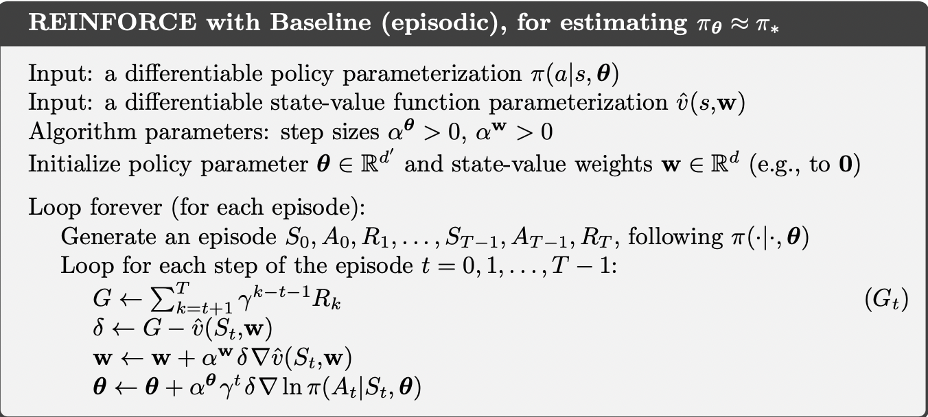
A simple approach uses MC estimates to estimate \(Q^{\pi_{\theta}} (X, A)\). This would lead to what is known as the REINFORCE algorithm:

In the on-policy setting when agent follows \(\pi_{\theta}\):

• It generates the sequence \(X_1, A_1, R_1\) with \(A_{t} \sim \pi_{\theta} (\cdot | X_t), X_t \sim \rho^{\pi_{\theta}}\).
• Then \(G_{t}^{\pi_{\theta}} = \sum_{k \geq t} \gamma^{k - t} R_{k}\) is an unbiased estimator of \(Q^{\pi_{\theta}} (X_t, A_t)\).
• We replace the action-value function with the estimate.
• The return however has high variance even though it is unbiased.
• We can use a state dependent baseline function (usually the value function) to reduce the variance.

Implementation

题目库: [242, 205, 215, 347, 349, 148, 1122, 973, "jz45", 147, 56, 57, 922, 104, 100, 101, 17, 102, 200, 98, 111, 112 103, 199, 994, 114]

Strings

242 Easy

先排序再比较就行，或者我们可以统计每个字母出现次数，关键是要明白字符数量不同就不相同

1
2
3
4
5

class Solution:
    def isAnagram(self, s: str, t: str) -> bool:
        s = sorted(s)
        t = sorted(t)
        return s == t

205 Easy

1
2
3
4
5
6
7
8
9
10
11
12
13
14
15
16
17
18

class Solution:
    def isIsomorphic(self, s: str, t: str) -> bool:
        if len(s) != len(t):
            return False
        mapping_s = {}
        mapping_t = {}
        for i, j in zip(s, t):
            if i not in mapping_s.keys():
                mapping_s[i] = j
                if j in mapping_t.keys():
                    return False
                mapping_t[j] = i

            else:
                if mapping_s[i] != j:
                    return False

        return True

Layer Normalization

Unlike Batch normalization, layer normalization directly estimates the normalization statistics from the summed inputs (multiply part of activation) to the neurons within a hidden layer, so the normalization does not introduce any new dependencies between training cases.

Notations

A feed-forward neural network is a non-linear mapping from a input pattern \(\mathbf{x}\) to an output vector \(\mathbf{y}\). Let \(\mathbf{a}^l\) be the vector representation of the summed inputs to the neurons in \(l\)th layer. It is computed by the weight matrix \(W^l = [w_1, ...., w_{N^l}]\) and previous input \(h^l\):

\[a_i^{l} = {w^{l}_i}^T h^l \;\;\;\;\;\;\;\; h_i^{l+1} = f(a_i^l + b_i^l)\]

where \(f(\cdot)\) is an element-wise non-linear activation function \(b_i^l\) is the scalar bias parameter. Batch normalization normalizes the summed inputs (multiply part of activation) to each hidden unit (\(a\) + bias) over the training cases:

\[\bar{a}_i^l = \frac{g_i^l}{\sigma_i^l} (a_i^l - \mu_i^l) \;\;\;\;\;\;\;\;\; \mu^l_i = \mathbb{E}_{\mathbf{x} \sim P(\cdot)} [a^l_i] \;\;\;\;\;\;\;\;\; \sigma_i^l = \sqrt{\mathbb{E}_{\mathbf{x} \sim P(\cdot)} [(a^l_i - \mu_i^l)^2]}\]

Where \(\bar{a}_i^l\) is the normalized summed inputs of \(i\)th activation, \(g_i\) is the scale parameter (\(\gamma_i\) in BN paper). The expectation is over the whole training data, in reality, we use samples from this expectation (mini-batch) to estimate the variance and mean.

In standard RNN, the summed inputs in the recurrent layer are computed from the current input \(\mathbf{x}^t\) (one sample) and previous vector of hidden states \(\mathbf{h}^{t-1}\):

\[\mathbf{a}^{t} = W_{hh}^T \mathbf{h}^{t-1} + W_{xh}^T\mathbf{x}^t\]

Where \(W_{hh}\) is the recurrent hidden to hidden wights and \(W_{xh}\) is the input to hidden weights.

Policy Search Methods (Policy Gradient)

All \(\nabla\) refer to \(\nabla_{\theta}\) for simplicity.

From introduction blog, our goal:

\[\underset{\pi_{\theta}}{\operatorname{maximize}} J_\rho(\pi_\theta) = \underset{\theta}{\operatorname{maximize}} J_\rho(\pi_\theta)\]

By taking the gradient w.r.t \(\theta\), we have:

We can swap integral and derivative as long as \(V^{\pi_{\theta}}\) is a continuous function of \(\theta\), the estimator of this expectation is called pathwise derivative estimator or stochastic backpropagation estimator (more details in Stochastic Graph).

This \(\nabla J_\rho(\pi_\theta)\) is called the Policy Gradient. In ideal case, if we know the policy gradient (i.e if we know the environment dynamics \(P, R\)), we can use gradient ascent to update the parameters \(\theta\).

Gradient Estimation Using Stochastic Computation Graphs

The backpropagation algorithm is only sufficient when the loss function is a deterministic, differentiable function of the parameter vector. The main practical result of this article is that to compute the gradient estimator, one just needs to make a simple modification to the backpropagation algorithm, where extra gradient signals are introduced at the stochastic nodes.

Preliminaries

Gradient Estimators for a Single Random Variable

Suppose \(X\) is a random variable, \(f\) is a function, we are interested in computing

\[\frac{\partial}{\partial \theta} E_{X}[f(X)]\]

There are few different ways that the process for generating \(X\) could be parameterized in terms of \(\theta\), which lead to different gradient estimators.

• We might be given a parameterized probability distribution \(X \sim p(\cdot ; \theta)\). In this case, we can use score function or REINFORCE or likelihood ratio estimator estimator:

  \[\frac{\partial}{\partial \theta} E_{X \sim p(\cdot ; \theta)}[f(X)] = \int_x \frac{\frac{\partial}{\partial\theta} p(x; \theta)}{p(x; \theta)} p(x; \theta) f(x)dx = E_{X \sim p(\cdot ; \theta)}[f(X) \frac{\partial}{\partial\theta} log p(X; \theta)]\]

  This equation is valid if \(p(x; \theta)\) is a continuous function of \(\theta\); however it does not need to be a continuous function of \(x\)

• \(X\) may be a deterministic, continuous function of \(\theta\) and another random variable \(Z\), we can write as \(X(\theta, Z)\). Then we can use the pathwise derivative or stochastic backpropagation estimator:

  \[E_{Z}[f(X(\theta, Z))] = E_{Z}[\frac{\partial}{\partial \theta} f(X(\theta, Z))]\]

  We can swap the derivative and expectation iff \(f(X(\theta, Z))\) is a continuous function of \(\theta\) for all values of \(Z\). However, it is also sufficient that this function is almost-everywhere differentiable.

• Finally, \(\theta\) may be appeared both in the probability distribution and inside the expectation:

  \[E_{Z \sim p(\cdot; \theta)}[f(X(\theta, Z))] = \int_z \frac{\partial}{\partial \theta} f(X(\theta, z)) p(z; \theta) dz = E_{Z \sim p(\cdot; \theta)}[\frac{\partial}{\partial \theta} f(X(\theta, Z)) + (\frac{\partial}{\partial \theta} log p(Z; \theta))f(X(\theta, Z))]\]

Batch Normalization: Accelerating Deep Network Training by Reducing Internal Covariate Shift

Internal covariate shift describes the phenomenon in training DNN that the distribution of each layer's inputs changes during training, as the parameters of the previous layer change. This slow down the training by requiring lower learning rates and careful parameter initialization, and makes it notoriously hard to train models with saturating non-linearities (tanh, sigmoid). This problem can be addressed by normalizing the layer inputs.

Introduction

To see the input distribution shift in terms of sub-network or a layer. Consider a network computing:

\[l = F_2(F_1(\textbf{u}, \Theta_1), \Theta_2)\]

Where \(F_1\) and \(F_2\) are arbitrary transformations, and the parameters \(\Theta_1, \Theta_2\) are to be learned to minimize the loss \(l\). Learning \(\Theta_2\) can be viewed as if inputs \(\textbf{x} = F_1(\textbf{u}, \Theta_1)\) and fed into the sub-network:

\[l = F_2(\textbf{x}, \Theta_2)\]

Thus, a fixed input distribution (ie. the distribution of \(\textbf{x}\)) would make the training more effective, because \(\Theta_2\) does not need to adapt to the new distribution. At the same time, if the mapping \(F_2\) is saturating non-linearity, a fixed-distribution will help to prevent the gradient of parameters from vanishing.